Todd-Coxeter algorithm and uniform polytopes
This project uses Python and POV-Ray to render 3D/4D uniform
polytopes. The code is hosted on GitHub
and requires the numpy library and the free raytracer,
POV-Ray.
Examples
All the images and videos displayed below are created using this program. The polytope data is computed in Python and then exported to POV-Ray for rendering.
All Platonic solids and Archimedean solids, prims and antiprisms, for example the snub dodecahedron:
All Kepler-Poinsot solids, for example the great icosahedron:
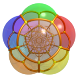
All uniform 4d polytopes (except the grand antiprism, which is non-Wythoffian), for example my github favicon, the runcinated 120-cell:
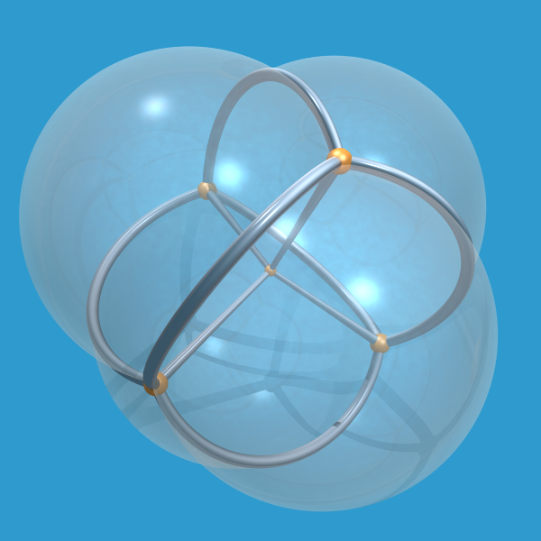
5-cell:
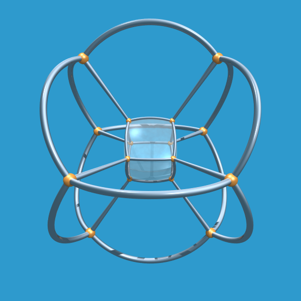
4d cube:
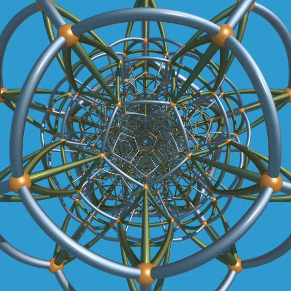
600-cell: (you can render the bubble faces and choose which of them are shown)
-
You can also render uniform star 4d polytopes, for example the grand stellated 120-cell:
and its rectified version (rendered in a curved fashion):
And finally, uniform 5D polytopes like 5-cube:
What are these examples about?
The polytopes showcased above are convex and non-convex uniform polytopes in 3D or 4D Euclidean spaces. Key terms to note include “convex/non-convex”, “Euclidean”, and “uniform”.
The term “convex” refers to the property of a polytope such that any line segment joining two points on the polytope lies entirely within the enclosure of the polytope. Examples of convex polytopes include Platonic solids, Archimedean solids, and Catalan solids, while non-convex ones include Kepler-Poinsot solids and star polychora.
In 3D Euclidean space, there are 18 different convex uniform polytopes (excluding the two infinite classes of prisms and antiprisms) and 57 different non-convex uniform polytopes. Currently, my program can only render the convex ones and a few non-convex ones, but I’m working on figuring out how to make it work for all of them in the future.
The term “Euclidean” is emphasized here because we also have uniform polytopes in other metric spaces, such as the hyperbolic metric, which bends the space and makes the polytopes look “deformed”. A famous example of this is the logo “Spikey” of Mathematica, which is based on the dodecahedron in hyperbolic 3-space.

The term “uniform” requires some mathematical subtleties. Roughly speaking, it means that
- All vertices are the same.
- All faces are regular polygons.
- All cells are uniform polyhedra (a polyhedron that satisfies conditions 1 and 2).
To explain what “the same” means, we need to use terms from group theory: it means that the symmetry group \(G\) of the polytope acts transitively on the set of vertices, such that for any pair of vertices \(u\) and \(v\), there is some \(g\in G\) that transforms \(u\) to \(v\): \(g \cdot u = v\).
In the above examples, the polytopes are colored such that all vertices, edges, and faces that are in the same orbit under the action of the symmetry group have the same color.
How to compute the data of a uniform polytope
Though these polytopes appear quite different from each other, they can all be constructed using a uniform approach called the Wythonff construction (also known as the kaleidoscope construction). In principle, this construction works in the same way as a kaleidoscope: we place reflection planes (mirrors) in space, passing through the origin and with carefully chosen angles between them (which must be of the form \(\pi-\pi/p\) for some rational \(p\)). These mirrors partition space into “rooms”. We choose any room (called the fundamental domain) and an initial vertex \(v_0\) in it, and then repeatedly reflect \(v_0\) about the mirrors to obtain a set of virtual images. All virtual images together with \(v_0\) form the vertices of our polytope. If \(v_1\) is the virtual image of \(v_0\) about the \(i\)-th mirror, then \((v_0,v_1)\) form an edge of type \(i\). We can use the symmetry group to transform it to other edges in the same orbit. Also, if \(v_0\) is firstly reflected about mirror \(i\) and then reflected about mirror \(j\), then since the composition of two reflections is a rotation, \(v_0\) is rotated about the center of some face \(f\) by an angle of \(2\pi/m\) (assuming the angle between mirror \(i\) and mirror \(j\) is \(\pi-\pi/m\)). We can recover \(f\) by applying this rotation \(m\) times and using the symmetry group to obtain other faces.
To implement the above strategy in a practical program, we need to address two main issues:
- How to position the mirrors and select the initial vertex \(v_0\) for a given convex uniform polytope?
- Once the mirrors and \(v_0\) are determined, how do we compute all the virtual images of \(v_0\)?
The solution to the first problem is known as the Coxeter-Dynkin diagram, which is a labeled undirected graph that encodes all the necessary information. Each uniform polytope has a corresponding Coxeter-Dynkin diagram that represents it, although different diagrams may represent the same polytope.
For example, the Coxeter-Dynkin diagram of the cube is:

Let’s delve deeper into the Coxeter-Dynkin diagram. Each node in the diagram represents a mirror in the kaleidoscope. In the diagram above, there are three nodes, and therefore three mirrors, which we label from left to right as \(m_0\), \(m_1\), and \(m_2\). The labelled edge between two nodes encodes the angle between their corresponding mirrors, as follows:
- Two nodes are connected if and only if the angle between their mirrors is not equal to \(\pi/2\).
- Two nodes are connected by an unlabelled edge if and only if the angle between their mirrors equals \(\pi-\pi/3\).
- Two nodes are connected by an edge labelled with a rational number \(m>2\) and \(m\ne3\) if and only if the angle between their mirrors equals \(\pi-\pi/m\).
Moreover, we use “circled” nodes to indicate which mirrors are “active”, i.e., those that do not contain the initial vertex \(v_0\). In this case, reflecting \(v_0\) about an active mirror produces a virtual image.
In the above example we have \(\langle m_0,m_1\rangle=\pi-\pi/4\), \(\langle m_1,m_2\rangle=\pi-\pi/3\), \(\langle m_0,m_2\rangle=\pi/2\). \(m_0\) is active, but \(m_1\) and \(m_2\) are not.
Therefore, we can place the three mirrors as follows: (\(n_i\) is the normalized normal vector of mirror \(m_i\))
- The normal of \(m_0\) can be chosen arbitrarily, for example \(n_0=(1,0,0)\).
- The angle between \(n_1\) and \(n_0\) is \(3\pi/4\), so we can choose \(n_1\) to be \(n_1=(\cos\dfrac{3\pi}{4}, \sin\dfrac{3\pi}{4}, 0)\).
- The normal of \(m_2\) is perpendicular to \(n_0\), so \(n_2\) has the form \((0,y_3,z_3)\). Using \(\langle n_1,n_2\rangle=2\pi/3\), we have \(y_3\sin\dfrac{3\pi}{4}=\cos\dfrac{2\pi}{3}\), and since \(z_3\) is a unit vector, \(z_3=\sqrt{1−y_3^2}\). We can solve these two equations to obtain \(y_3,z_3\).
To choose an initial vertex \(v_0\) that lies on both \(m_1\) and \(m_2\) but not on \(m_0\), we can choose \(v_0\) so that its distance to \(m_0\) is 1 and its distance to \(m_1\) and \(m_2\) are both 0:
\[\begin{align*}\langle v_0, n_0\rangle=1,\\\langle v_0, n_1\rangle=0,\\\langle v_0, n_2\rangle=0.\\\end{align*}\]
Then solve this linear system to get \(v_0\).
As mentioned before the angles between the mirrors must be chosen carefully to ensure \(v_0\) and its virtual images form the vertices of an uniform polytope, this restricts us to only finitely many choices of Coxeter diagrams, you can refer to this wiki page for the complete list.
The answer to the second question is called the Todd-Coxeter algorithm, I’ll discuss it in the next section.
Finitely presented groups and Todd-Coxeter algorithm
How can we obtain all the virtual images of the initial vertex \(v_0\) with respect to all mirrors? An obvious but crude method is to repeatedly reflect \(v_0\) about the mirrors and compare the resulting images with the set of virtual images obtained so far (within a predefined rounding error bound) until no new virtual images emerge. This approach is easy to program but it’s unappealing from a mathematician’s perspective, as it fails to utilize the abundant symmetries inherent in the polytope.
This program takes a “symbolic computation” approach by solving the coset enumeration problem in the symmetry group. It offers the advantage of providing exact information about the polytope without resorting to rounding errors or approximation procedures. However, the price we pay is that the math involved is somewhat complex (and hence so is the code), and readers should have some basic knowledge of group theory to understand it.
Firstly, let’s recall the orbit-stabilizer theorem from group theory:
Theorem: Suppose a group \(G\) acts transitively on a set \(S\), and let \(x \in S\) have stabilizer subgroup \(H \leq G\). Then there exists a one-to-one correspondence between \(S\) and the right cosets of \(G/H\): \(x \cdot g \mapsto Hg\).
Note that the action of \(G\) on \(S\) is written as “applying on the right”, this is mainly for programming convenience and has no significant difference from applying on the left.
The theorem mentioned above tells us that if a group \(G\) acts transitively on a set \(S\) and we know the stabilizing subgroup of some \(x\in S\) in \(G\) is \(H\), then we can recover the entire orbit \(S\) by applying a set of coset representatives of \(G/H\) to \(x\).
Therefore, to compute all vertices of a given uniform polytope \(P\), we can follow these steps:
- Obtain a presentation of the symmetry group \(G\) and the coordinates of an initial vertex \(v_0\) from the Coxeter-Dynkin diagram.
- Obtain a presentation of the stabilizing subgroup \(H\) of \(v_0\) in \(G\) and calculate a set of right coset representatives of \(G/H\).
- Apply these representatives to \(v_0\) to obtain all vertices of \(P\).
Again we use the cube as an example to show this procedure: recall the Coxeter-Dynkin diagram of the cube is
The mirrors of the cube are \(m_0, m_1,\) and \(m_2\), with normals \(n_0, n_1,\) and \(n_2\), respectively, all of which are unit vectors. The reflections about these mirrors are denoted as \(\rho_0, \rho_1,\) and \(\rho_2\), and the matrix of \(\rho_i\) is \(M_i = I - 2n_in_i^T\) (see Householder transformation).
The symmetry group \(G\) of the cube is generated by the three aforementioned “generator reflections”: \(\rho_0, \rho_1,\) and \(\rho_2\). A presentation of the group is:
\[G = \langle\rho_0,\rho_1,\rho_2\ |\ \rho_0^2=\rho_1^2=\rho_2^2=(\rho_0\rho_1)^4=(\rho_1\rho_2)^3=(\rho_0\rho_2)^2=1\rangle.\]
This is because a reflection always has order 2 and since \(\rho_0\) and \(\rho_1\) are two reflections with an angle of \(3\pi/4\) between their mirrors, \(\rho_0\rho_1\) is a rotation about the line of intersection of their mirrors with an angle of \(3\pi/2\). Therefore, \((\rho_0\rho_1)^4=1\). Similarly, we have the relations for \(\rho_1\rho_2\) and \(\rho_0\rho_2\).
Note: It is natural to wonder if we might be missing some “hidden” relations. For convex polytopes, the answer is no, but for certain star polytopes, the answer is yes. In these cases, we need to add extra relations to ensure the procedure works correctly. A significant difference is that, in convex cases, the symmetry group always maps the interior of the fundamental domain to another disjoint one, whereas in star polytopes, the fundamental domain may be covered multiple times by other domains. For more information, refer to Vinberg’s paper “Discrete linear groups generated by reflections”.
One can employ the Todd-Coxeter algorithm (which will be explained later) to calculate a comprehensive list of all 48 elements in \(G\).
\[\begin{array}{lll}e&\rho_{0}&\rho_{0}\rho_{1}\\\rho_{0}\rho_{1}\rho_{0}&\rho_{0}\rho_{1}\rho_{0}\rho_{1}&\rho_{1}\rho_{0}\rho_{1}\\\rho_{1}\rho_{0}&\rho_{1}&\rho_{0}\rho_{2}\\\rho_{2}&\rho_{1}\rho_{2}&\rho_{1}\rho_{2}\rho_{1}\\\rho_{2}\rho_{1}&\rho_{0}\rho_{1}\rho_{2}&\rho_{0}\rho_{1}\rho_{2}\rho_{1}\\\rho_{0}\rho_{2}\rho_{1}&\rho_{0}\rho_{1}\rho_{0}\rho_{2}&\rho_{0}\rho_{1}\rho_{0}\rho_{1}\rho_{2}\\\rho_{0}\rho_{1}\rho_{0}\rho_{1}\rho_{2}\rho_{1}&\rho_{0}\rho_{1}\rho_{0}\rho_{2}\rho_{1}&\rho_{1}\rho_{0}\rho_{1}\rho_{2}\\\rho_{1}\rho_{0}\rho_{2}&\rho_{1}\rho_{0}\rho_{2}\rho_{1}&\rho_{1}\rho_{0}\rho_{1}\rho_{2}\rho_{1}\\\rho_{2}\rho_{1}\rho_{0}&\rho_{2}\rho_{1}\rho_{0}\rho_{1}&\rho_{0}\rho_{2}\rho_{1}\rho_{0}\rho_{1}\\\rho_{0}\rho_{2}\rho_{1}\rho_{0}&\rho_{1}\rho_{0}\rho_{2}\rho_{1}\rho_{0}&\rho_{1}\rho_{0}\rho_{2}\rho_{1}\rho_{0}\rho_{1}\\\rho_{1}\rho_{2}\rho_{1}\rho_{0}\rho_{1}&\rho_{1}\rho_{2}\rho_{1}\rho_{0}&\rho_{0}\rho_{1}\rho_{0}\rho_{2}\rho_{1}\rho_{0}\\\rho_{0}\rho_{1}\rho_{0}\rho_{2}\rho_{1}\rho_{0}\rho_{1}&\rho_{0}\rho_{1}\rho_{2}\rho_{1}\rho_{0}\rho_{1}&\rho_{0}\rho_{1}\rho_{2}\rho_{1}\rho_{0}\\\rho_{1}\rho_{0}\rho_{1}\rho_{2}\rho_{1}\rho_{0}&\rho_{1}\rho_{0}\rho_{1}\rho_{2}\rho_{1}\rho_{0}\rho_{1}&\rho_{0}\rho_{1}\rho_{0}\rho_{1}\rho_{2}\rho_{1}\rho_{0}\rho_{1}\\\rho_{0}\rho_{1}\rho_{0}\rho_{1}\rho_{2}\rho_{1}\rho_{0}&\rho_{2}\rho_{1}\rho_{0}\rho_{1}\rho_{2}&\rho_{1}\rho_{2}\rho_{1}\rho_{0}\rho_{1}\rho_{2}\\\rho_{0}\rho_{2}\rho_{1}\rho_{0}\rho_{1}\rho_{2}&\rho_{0}\rho_{1}\rho_{2}\rho_{1}\rho_{0}\rho_{1}\rho_{2}&\rho_{1}\rho_{0}\rho_{2}\rho_{1}\rho_{0}\rho_{1}\rho_{2}\\\rho_{1}\rho_{0}\rho_{1}\rho_{2}\rho_{1}\rho_{0}\rho_{1}\rho_{2}&\rho_{0}\rho_{1}\rho_{0}\rho_{2}\rho_{1}\rho_{0}\rho_{1}\rho_{2}&\rho_{0}\rho_{1}\rho_{0}\rho_{1}\rho_{2}\rho_{1}\rho_{0}\rho_{1}\rho_{2}\end{array}\]
Since the initial vertex \(v_0\) is on \(m_1\) and \(m_2\) but not on \(m_0\) in the Coxeter-Dynkin diagram, only the mirror \(m_0\) is active. Thus, both \(\rho_1\) and \(\rho_2\) map \(v_0\) to itself, while \(\rho_0\) maps \(v_0\) to its virtual image about \(m_0\). Therefore, the stabilizing subgroup of \(v_0\) is given by:
\[H=\langle \rho_1, \rho_2\ |\ \rho_1^2=\rho_2^2=(\rho_1\rho_2)^3=e\rangle.\]
Note: You may wonder if we can only claim that the subgroup generated by \({\rho_0,\rho_1}\) is contained in the stabilizing subgroup of \(v_0\) but may not be exactly equal to it. Indeed, this is a possibility. However, for Coxeter groups, it is a property that in the geometric realization of a Coxeter group \(W\) (that is, representing \(W\) as a set of reflections about hyperplanes in \(\mathbb{R}^n\)), the stabilizing subgroup of any point \(v\) in the fundamental domain is a standard parabolic subgroup generated by those simple reflections whose hyperplanes contain \(v\). This may seem like an obvious geometric intuition, but it requires a quite non-trivial proof, which can be found in Humphreys’s book “Reflection Groups and Coxeter Groups”, chapter 1.
It is clear that \(H\) is the dihedral group \(D_3\), thus \(|H|=6\) and \(|G/H|=8\). Using the Todd-Coxeter algorithm, we can obtain a complete list of coset representatives for \(G/H\):
\[\begin{array}{llll}e&\rho_{0}&\rho_{0}\rho_{1}&\rho_{0}\rho_{1}\rho_{0}\\\rho_{0}\rho_{1}\rho_{2}&\rho_{0}\rho_{1}\rho_{0}\rho_{2}&\rho_{0}\rho_{1}\rho_{0}\rho_{2}\rho_{1}&\rho_{0}\rho_{1}\rho_{0}\rho_{2}\rho_{1}\rho_{0}\end{array}\]
Applying these coset representatives to \(v_0\) gives us the 8 vertices of the cube. For example, the action of \(\rho_0\rho_1\) on \(v_0\) is as follows:
\[v_0(\rho_0\rho_1)=(v_0\rho_0)\rho_1=(v_0M_0)\rho_1=v_0M_0M_1.\]
Here, \(v_0\) is represented as a row vector since all \(M_i\)’s are symmetric matrices.
We can also use the same procedure to find all edges and faces of the cube. To find all edges of type \(i\), we proceed as follows:
- Check if the initial vertex \(v_0\) lies on the mirror \(m_i\). If it does, then the reflection \(\rho_i\) fixes \(v_0\), and there are no edges of type \(i\). Otherwise, let \(v_1=\rho_i(v_0)\). Then, the segment \((v_0,v_1)\) forms an edge \(e\) of type \(i\)
- To find the stabilizing subgroup of \(e\), we note that a symmetry fixes \(e\) if and only if it fixes the midpoint \(p\) of \(e\). Thus, the stabilizing subgroup of \(e\) is the same as the stabilizing subgroup of \(p\). From the previous comment, we know that this subgroup is generated by those simple reflections whose mirrors contain \(p\). These mirrors are either \(m_i\) (bisects \(e\)), or those containing \(v_0\) and orthogonal to \(m_i\) (contain \(e\)), so the stabilizing subgroup of \(e\) is generated by \(\rho_i\) and those simple reflections that fix \(v_0\) and commute with \(\rho_i\). In the case of the cube, we have \(H=\langle \rho_0,\rho_2\rangle\), so \(|H|=4\) and \(|G/H|=12\), confirming that the cube has 12 edges.
- We then find a set of coset representatives of \(G/H\) and apply them to \(e\) to obtain all edges of type \(i\).
To find all faces of type \((i,j)\), where \(i\neq j\), we use the same procedure. If at least one of \(m_i,m_j\) is active, then the rotation \(r_{ij}=\rho_i\rho_j\) generates a face \(f\) of type \((i,j)\), which is invariant under \(\rho_i\) and \(\rho_j\). However, if \(v_0\) lies on exactly one of the two mirrors and they are perpendicular, we need to be careful. In this case, the stabilizing subgroup of \(f\) is generated by \(\rho_i\), \(\rho_j\), and those generators that fix \(v_0\) and commute with both \(\rho_i\) and \(\rho_j\). We then find a set of coset representatives of \(G/H\) and apply them to \(f\) to obtain all faces of type \((i,j)\).
Now the key step is to compute a set of coset representatives of \(G/H\) for a finitely presented group \(G\) and its subgroup \(H\), which is exactly what the Todd-Coxeter algorithm does.
The Todd-Coxeter algorithm can be thought of as a Sudoku game where the table to complete is a dynamically growing 2D array \(T\). The rows of \(T\) are labeled by the right cosets in \(G/H\), and the columns of \(T\) are labeled by the generators of \(G\). Each entry \(T[i][j]\) records the right coset obtained by multiplying the \(j\)-th generator on the right of the \(i\)-th coset. The algorithm uses the defining relations in the presentation of \(G\) and \(H\) as guidelines to find new cosets and fill their corresponding entries in \(T\). The game ends when all entries in \(T\) are filled, and the coset in each entry has a row in \(T\) and satisfies all relations. The resulting \(T\) is the adjacency matrix of the Schreier graph of \(G/H\), and one can easily obtain a complete list of word representations for all cosets in \(G/H\).
For a more detailed treatment of the Todd-Coxeter algorithm, please refer to the Handbook of Computational Group Theory (HCGT) or other related literature.
Chapter 5, Handbook of Computational Group Theory, Holt, D., Eick, B., O’Brien, E.
I will demonstrate below how the algorithm works using the cube as an example:
Example: let \(G\) be the symmetric group of the cube: \[\begin{align*}G = \langle\rho_0,\rho_1,\rho_2\ |\ \rho_0^2&=\rho_1^2=\rho_2^2=(\rho_0\rho_1)^4=(\rho_1\rho_2)^3\\&=(\rho_0\rho_2)^2=1\rangle.\end{align*}\] and subgroup \(H=\langle \rho_1, \rho_2\rangle\). Find a set of coset representatives of \(G/H\).
Our known relations:
- For each generator word \(w\) of \(H\), it holds \(Hw=H\), i.e. \(H\rho_1=H\) and \(H\rho_2=H\).
- For any coset \(K\) and any generator relation \(r\) of \(G\) it holds \(Kr=K\), i.e. \(K\rho_i^2=K,i=0,1,2\), and \(K(\rho_0\rho_1)^4=K(\rho_1\rho_2)^3=K(\rho_0\rho_2)^2=K.\)
These relations can be stored in two lists, one for the relations in \(H\) and one for the relations in \(G\), each relation can be further stored as an array of int type.
The first list stores the generator words of \(H\):
- (1,) // \(\rho_1\)
- (2,) // \(\rho_2\)
The second list stores the defining relations of \(G\):
- (0, 0) // \(\rho_0^2=1\)
- (1, 1) // \(\rho_1^2=1\)
- (2, 2) // \(\rho_2^2=1\)
- (0, 1, 0, 1, 0, 1, 0, 1) // (\(\rho_0\rho_1)^4=1\)
- (1, 2, 1, 2, 1, 2) // (\(\rho_1\rho_2)^3=1\)
- (0, 2, 0, 2) // (\(\rho_0\rho_2)^2=1\)
The relations are numbered from 0 to 7 for easy reference in the following steps.
Note: When \(G\) is not represented as a Coxeter group, for example in the case of snub polytopes, we need to consider the inverse of the generators as well, and they also occupy their own columns in \(T\). Therefore, the actual number of columns in \(T\) is twice the number of generators. However, for Coxeter groups, all generators are involutions, so there is no need to insert columns for their inverses.
Initially, the table \(T\) has only one row, corresponding to the coset \(H\) (which is the only coset we know at this point).
| \(\phantom{}\) | \(\rho_0\) | \(\rho_1\) | \(\rho_2\) |
|---|---|---|---|
| \(H_0\) | \(\phantom{}\) | \(\phantom{}\) | \(\phantom{}\) |
Here, the algorithm initializes \(H_0\) to be the subgroup \(H\) and checks if it satisfies all relations in the first list. Once this check is done, the first list can be discarded. Then, the algorithm scans all cosets of \(T\) from top to bottom and verifies if the current coset satisfies all relations in the second list. During this process, new cosets may be defined and their rows are appended at the end of \(T\). However, it is important to note that some cosets in the table may actually represent the same coset, so care must be taken.
Let’s start by scanning \(H_0\) and checking whether the relations in the first list are satisfied by it:
- For relation 0, we have \(H_0\rho_1=H_0\), i.e., \(T[0][1]=0\).
- For relation 1, we have \(H_0\rho_2=H_0\), i.e., \(T[0][2]=0\).
\(T\) is now updated as follows:
| \(\phantom{}\) | \(\rho_0\) | \(\rho_1\) | \(\rho_2\) |
|---|---|---|---|
| \(H_0\) | \(\phantom{}\) | 0 | 0 |
Now that \(H_0\) satisfies all relations in the first list, we can discard it and focus on checking the relations in the second list.
We move on to check the relations in the second list for \(H_0\):
(2). Relation 2 says \(H_0\rho_0^2=H_0\). Since we do not know \(H_0\rho_0\) yet, we define it to be \(H_1\), fill in 1 in its entry \(T[0][0]\), and append a new row for \(H_1\):
| \(\phantom{}\) | \(\rho_0\) | \(\rho_1\) | \(\rho_2\) |
|---|---|---|---|
| \(H_0\) | 1 | 0 | 0 |
| \(H_1\) | 0 | \(\phantom{}\) | \(\phantom{}\) |
Note that each time we define or find \(H_i\rho_j=H_k\) for some \(i,j,k\), we automatically get the “dual” relation \(H_k\rho_j=H_i\). Therefore, we always fill in a pair of entries \(T[i][j]=k\) and \(T[k][j]=i\) at a time.
(3). Relations 3 and 4 are already satisfied, so we continue.
(4). Relation 5 says \(H_0\rho_0\rho_1\rho_0\rho_1\rho_0\rho_1\rho_0\rho_1=H_0\). We already know \(H_0\rho_0=H_1\), but \(H_1\rho_1\) is unknown, so we define it to be \(H_2\). We fill in the two entries \(T[1][3]=2\) and \(T[2][3]=1\) and append a new row for \(H_2\).
| \(\phantom{}\) | \(\rho_0\) | \(\rho_1\) | \(\rho_2\) |
|---|---|---|---|
| \(H_0\) | 1 | 0 | 0 |
| \(H_1\) | 0 | 2 | \(\phantom{}\) |
| \(H_2\) | \(\phantom{}\) | 1 | \(\phantom{}\) |
\(H_2\rho_0\) is not yet defined, so we set \(H_2\rho_0=H_3\) and update the corresponding entries in \(T\):
| \(\rho_0\) | \(\rho_1\) | \(\rho_2\) | |
|---|---|---|---|
| \(H_0\) | 1 | 0 | 0 |
| \(H_1\) | 0 | 2 | \(\phantom{}\) |
| \(H_2\) | 3 | 1 | \(\phantom{}\) |
| \(H_3\) | 2 | \(\phantom{}\) | \(\phantom{}\) |
Continuing with the scan, we notice that \(H_3\rho_1\) is unknown, and we might be tempted to define it as a new coset \(H_4\) and continue. However, this strategy can create many redundant cosets, leading to a rapid growth of \(T\). Instead, we scan the relation in reverse order, trying to fill the gaps without introducing new cosets. Recall that we scanned from left to right, and we arrived at the following position: \[H_0\rho_0\rho_1\rho_0(=H_3)\rho_1\rho_0\rho_1\rho_0\rho_1=H_0.\] Now, scanning from right to left, we get \(H_0\rho_1\rho_0\rho_1\rho_0=H_3\), which means that \[H_0\rho_0\rho_1\rho_0(=H_3)\rho_1 =H_0\rho_1\rho_0\rho_1\rho_0=H_3.\] Thus, we have deduced that \(H_3\rho_1=H_3\), instead of defining it as a new coset. This technique is called a deduction, as described in the book HCGT. Therefore, we update \(T\) accordingly:
| \(\phantom{}\) | \(\rho_0\) | \(\rho_1\) | \(\rho_2\) |
|---|---|---|---|
| \(H_0\) | 1 | 0 | 0 |
| \(H_1\) | 0 | 2 | \(\phantom{}\) |
| \(H_2\) | 3 | 1 | \(\phantom{}\) |
| \(H_3\) | 2 | 3 | \(\phantom{}\) |
So in the actual program we always scan a relation from both ends and define new cosets if necessary until they meet.
(5). Relation 6 is already satisfied, continue.
(6). Relation 7 says \(H_0\rho_0\rho_2\rho_0\rho_2=H_0\), scanning from both ends gives \[H_0\rho_0(=H_1)\rho_2=H_0\rho_2\rho_0=H_1,\] hence \(H_1\rho_2=H_1\) and we make another deduction. \(T\) now becomes
| \(\phantom{}\) | \(\rho_0\) | \(\rho_1\) | \(\rho_2\) |
|---|---|---|---|
| \(H_0\) | 1 | 0 | 0 |
| \(H_1\) | 0 | 2 | 1 |
| \(H_2\) | 3 | 1 | \(\phantom{}\) |
| \(H_3\) | 2 | 3 | \(\phantom{}\) |
Now, \(H_0\) satisfies all relations in the two lists and the scanning of the first row is completed. We can move on to begin scanning of the row for \(H_1\). Note the first list is now discarded, and we will only check relations 2-7.
(1). Relations 2, 3, 4, and 5 are already satisfied. We can continue to the next relation. (2). Relation 6 says \(H_1\rho_1\rho_2\rho_1\rho_2\rho_1\rho_2=H_1\). We know that \(H_1\rho_1=H_2\), but \(H_2\rho_2\) is unknown. Backward scanning also gets stuck here: \[H_1\rho_1(=H_2)\rho_2\rho_1=H_1\rho_2\rho_1\rho_2=H_2\rho_2.\] So we define \(H_2\rho_2=H_4\). Then we have \(H_4\rho_1=H_4\), and \(T\) becomes:
| \(\rho_0\) | \(\rho_1\) | \(\rho_2\) | |
|---|---|---|---|
| \(H_0\) | 1 | 0 | 0 |
| \(H_1\) | 0 | 2 | 1 |
| \(H_2\) | 3 | 1 | 4 |
| \(H_3\) | 2 | 3 | \(\phantom{}\) |
| \(H_4\) | \(\phantom{}\) | 4 | 2 |
- Relation 7 is already satisfied for \(H_1\), so we can move on to scan the row for \(H_2\).
I’ll leave it as an exercise for you to complete the scanning of \(H_2\), \(H_3\), \(H_4\), and \(H_5\). These are relatively easy tasks. Once \(H_2\) has been scanned, your \(T\) should look like this:
| \(\rho_0\) | \(\rho_1\) | \(\rho_2\) | |
|---|---|---|---|
| \(H_0\) | 1 | 0 | 0 |
| \(H_1\) | 0 | 2 | 1 |
| \(H_2\) | 3 | 1 | 4 |
| \(H_3\) | 2 | 3 | 5 |
| \(H_4\) | 5 | 4 | 2 |
| \(H_5\) | 4 | \(\phantom{}\) | 3 |
After completing the scanning of \(H_3\), your \(T\) should be:
| \(\rho_0\) | \(\rho_1\) | \(\rho_2\) | |
|---|---|---|---|
| \(H_0\) | 1 | 0 | 0 |
| \(H_1\) | 0 | 2 | 1 |
| \(H_2\) | 3 | 1 | 4 |
| \(H_3\) | 2 | 3 | 5 |
| \(H_4\) | 5 | 4 | 2 |
| \(H_5\) | 4 | 6 | 3 |
| \(H_6\) | \(\phantom{}\) | 5 | 6 |
After completing the scanning for \(H_4\), your \(T\) should be:
| \(\rho_0\) | \(\rho_1\) | \(\rho_2\) | |
|---|---|---|---|
| \(H_0\) | 1 | 0 | 0 |
| \(H_1\) | 0 | 2 | 1 |
| \(H_2\) | 3 | 1 | 4 |
| \(H_3\) | 2 | 3 | 5 |
| \(H_4\) | 5 | 4 | 2 |
| \(H_5\) | 4 | 6 | 3 |
| \(H_6\) | 7 | 5 | 6 |
| \(H_7\) | 6 | 7 | \(\phantom{}\) |
And when we scan \(H_6\), we find that relations 2-6 are already satisfied. From relation 7, \(H_6\rho_0\rho_2\rho_0\rho_2=H_6\), we get a deduction \(H_7\rho_2=H_7\), and \(T\) is updated as follows:
| \(\rho_0\) | \(\rho_1\) | \(\rho_2\) | |
|---|---|---|---|
| \(H_0\) | 1 | 0 | 0 |
| \(H_1\) | 0 | 2 | 1 |
| \(H_2\) | 3 | 1 | 4 |
| \(H_3\) | 2 | 3 | 5 |
| \(H_4\) | 5 | 4 | 2 |
| \(H_5\) | 4 | 6 | 3 |
| \(H_6\) | 7 | 5 | 6 |
| \(H_7\) | 6 | 7 | 7 |
One can check that \(H_7\) satisfies all relations in the second list, so no more cosets can be found and the game is over.
The multiplication relations between these cosets can be obtained using breadth-first search:
\[\begin{array}{l}H_0 = H_0\cdot e,\\ H_1=H_0\cdot\rho_0,\\H_2=H_1\cdot\rho_1=H_0\cdot\rho_0\rho_1,\\H_3=H_2\cdot\rho_0=H_0\cdot\rho_0\rho_1\rho_0,\\ H_4=H_2\cdot\rho_2=H_0\cdot\rho_0\rho_1\rho_2,\\ H_5=H_3\cdot\rho_2=H_0\cdot \rho_0\rho_1\rho_0\rho_2,\\ H_6=H_5\cdot\rho_1=H_0\cdot \rho_0\rho_1\rho_0\rho_2\rho_1,\\ H_7=H_6\cdot\rho_0=H_0\cdot \rho_0\rho_1\rho_0\rho_2\rho_1\rho_0.\end{array}\]
So a set of representatives can be chosen as
\[\begin{array}{llll}e&\rho_{0}&\rho_{0}\rho_{1}&\rho_{0}\rho_{1}\rho_{0}\\\rho_{0}\rho_{1}\rho_{2}&\rho_{0}\rho_{1}\rho_{0}\rho_{2}&\rho_{0}\rho_{1}\rho_{0}\rho_{2}\rho_{1}&\rho_{0}\rho_{1}\rho_{0}\rho_{2}\rho_{1}\rho_{0}\end{array} \] This is exactly what we have seen before.
Note: This example is a bit tedious, but it is still a simple one because we did not encounter the case where two cosets in the table are found to be the same (in the book HCGT, this is called a coincidence). When this occurs, the scanning must be paused, and the control flow is jumped to handle this coincidence: a new stack \(q\) is opened, and this pair of coincidences is pushed into \(q\). Then, one pair of coincidences is popped from \(q\) at a time, their rows are merged, and new coincidences that occur in the merging process are pushed into \(q\).
Snub polytopes
Snub polytopes can be constructed by applying rotations in the full symmetry group to the initial vertex \(v_0\). In the case of the cube, we have seen the full symmetry group \(G\) is
\[G = \langle\rho_0,\rho_1,\rho_2\ |\ \rho_0^2=\rho_1^2=\rho_2^2=(\rho_0\rho_1)^4=(\rho_1\rho_2)^3=(\rho_0\rho_2)^2=1\rangle.\]
\(G\) consists of 48 elements, half of which are rotations, so totaling 24 rotations. These rotations constitute the symmetry group \(\widetilde{G}\) of the snub cube, which can be generated by three fundamental rotations: \(r_0=\rho_0\rho_1\), \(r_1=\rho_1\rho_2\), and \(r_2=\rho_0\rho_2\). Since \(r_0r_1=r_2\), it follows that \(\widetilde{G}\) can be generated by only \(r_0\) and \(r_1\).
A presentation of \(\widetilde{G}\) is \[\widetilde{G}=\langle r_0,r_1\ |\ r_0^4=r_1^3=(r_0r_1)^2=1\rangle.\] Using the Todd-Coxeter algorithm, we can obtain a complete list of word representations of \(\widetilde{G}\):
\[\begin{array}{lll}e&r_{0}&r_{0}r_{0}\\r_{0}r_{0}r_{0}&r_{1}&r_{1}r_{1}\\r_{0}r_{1}&r_{0}r_{1}r_{1}&r_{0}r_{0}r_{1}\\r_{0}r_{0}r_{1}r_{1}&r_{0}r_{0}r_{0}r_{1}&r_{1}r_{0}\\r_{1}r_{0}r_{0}&r_{1}r_{0}r_{0}r_{0}&r_{1}r_{1}r_{0}\\r_{1}r_{1}r_{0}r_{0}&r_{0}r_{1}r_{1}r_{0}&r_{0}r_{1}r_{1}r_{0}r_{0}\\r_{0}r_{0}r_{1}r_{1}r_{0}&r_{1}r_{0}r_{0}r_{1}&r_{1}r_{0}r_{0}r_{1}r_{1}\\r_{1}r_{0}r_{0}r_{0}r_{1}&r_{1}r_{1}r_{0}r_{0}r_{1}&r_{0}r_{1}r_{1}r_{0}r_{0}r_{1}\end{array} \]
We choose the initial vertex \(v_0\) so that it’s not on any of the three mirrors, and apply the above word representations of \(\widetilde{G}\) to \(v_0\). This gives the 24 vertices of the snub cube.
To obtain the edges of the snub cube, the following steps can be taken:
- Each rotation \(r_i\,(i=0,1,2)\) generates a base edge \(e\). These base edges are in different orbits under the action of \(\widetilde{G}\).
- The stabilizing subgroup of \(e\) is \(H=\langle 1\rangle\) if the order of \(r_i\) is greater than 2, or the cyclic group \(H=\langle r_i\rangle\) if the order of \(r_i\) is 2. The coset representatives of \(G/H\) can be computed, and applied to \(e\) to obtain all other edges of type \(i\).
The case of faces is slightly more involved:
Each rotation \(r_i\,(i=0,1)\) generates a base face \(f={v_0, r_i(v_0),\ldots, r_i^{m-1}(v_0)}\) for \(m>2\), where \(m\) is the order of \(r_i\). For \(i=2\), \(m=2\), and \(f\) is degenerated to an edge. The stabilizing subgroup of \(f\) is the cyclic group \(H=\langle r_i\rangle\). The coset representatives of \(G/H\) can be computed, and applied to \(f\) to obtain all other faces of type \(i\). For the snub cube, there are \(6\) square faces generated by \(r_0\) (since \(24/|\langle r_0\rangle|=24/4=6\)), and \(8\) triangle faces generated by \(r_1\) (since \(24/|\langle r_1\rangle|=24/3=8\)).
There is another type of triangle faces which comes from the relation \(r_0r_1=r_2\). Let’s consider the three vertices \({v_0,v_0r_1,v_0r_2}\). We see that \((v_0, v_0r_1)\) is an edge of type 1 and \((v_0, v_0r_2)\) is an edge of type 2. But we also have \[(v_0, v_0r_0)\xrightarrow{\ r_1\ }(v_0r_1, v_0r_0r_1) = (v_0r_1, v_0r_2).\] That is, \((v_0r_1, v_0r_2)\) is an edge of type 0 obtained by applying \(r_1\) to the base edge \((v_0, v_0r_0)\). The stabilizing subgroup of this triangle must be \(\langle1\rangle\) since all its three edges are in different orbits. Thereforre, we have \(|\widetilde{G}|/1=24\) triangle faces of this “mixed type”, which are not generated by any of the “fundamental rotations”.
So the snub cube has \(6+8+24=38\) faces in total.
Star polytopes
Most star polytopes can be generated using the Wythoff construction, but generally, it is not enough to use the method described above directly. You also need to add an additional generating relation into the group’s presentation.
To illustrate, let’s take the great dodecahedron as an example. Its Coxeter-Dynkin diagram is shown below:

Therefore, the angles between the mirrors are \(\pi-2\pi/5, \pi/2, \pi-\pi/5\). If we continue with the previous analysis, we obtain the presentation of the symmetry group as:
\[K = \langle\tau_0,\tau_1,\tau_2 \ |\ \tau_0^2=\tau_1^2=\tau_2^2=(\tau_0\tau_1)^5=(\tau_1\tau_2)^5=(\tau_0\tau_2)^2=1\rangle. \]
This group is infinite, and since the quotient group of the stabilizer subgroup of \(v_0\) is also infinite, the Todd-Coxeter algorithm will not work here.
In fact, we just need to add another generating relation to the presentation, namely \((\tau_0\tau_1\tau_2\tau_1)^3=1\). With this addition, the presentation of the symmetry group becomes:
\[\begin{align*} K = \langle\tau_0,\tau_1,\tau_2 \ |\ &\tau_0^2=\tau_1^2=\tau_2^2=(\tau_0\tau_1)^5=(\tau_1\tau_2)^5=\\&(\tau_0\tau_2)^2=(\tau_0\tau_1\tau_2\tau_1)^3=1\rangle. \end{align*}\]
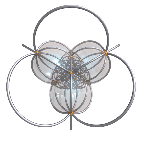
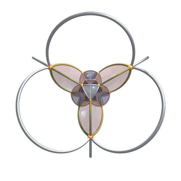
Note that I intentionally used \(\tau\) to represent reflections and \(K\) to denote the symmetry group of the great dodecahedron. What’s happening here? Let’s take a look at the video:
From the video, we can observe that the great dodecahedron and the icosahedron share the exact same set of vertices. However, it seems that the great dodecahedron can be obtained by digging some triangular holes on the surface of the icosahedron. In general, if the hole of a star-shaped polyhedron is a polygon with \(h\) sides, the corresponding extra relation is given by \((\tau_0\tau_1\tau_2\tau_1)^h=1\).
Let’s take a closer look at the fundamental region of the great dodecahedron:
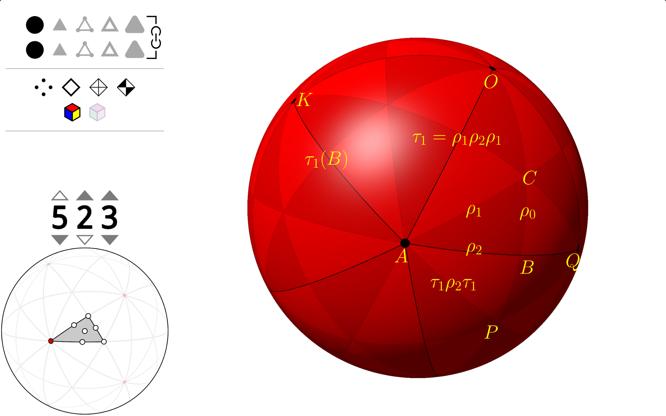
The figure above shows \(\Delta ABC\) as the fundamental domain of the icosahedron. Its internal angles are \(\angle CAB=\pi/5\),\(\angle CBA=\pi/2\),\(\angle ACB=\pi/3\). Reflections about the arcs \(BC\), \(AC\), and \(AB\) are denoted by \(\rho_0\), \(\rho_1\), and \(\rho_2\), respectively. The presentation of the symmetry group of icosahedron, \(G\), can be expressed as follows: \[G = \langle\rho_0,\rho_1,\rho_2\ |\ \rho_0^2=\rho_1^2=\rho_2^2=(\rho_0\rho_1)^3=(\rho_1\rho_2)^5=(\rho_0\rho_2)^2=1\rangle.\]
The great dodecahedron can be constructed as follows: we keep the vertices and edges of the icosahedron untouched, but change its faces. To do this we start a walk from vertex \(Q\) and move along edge \(QA\) to reach the next vertex \(A\). At \(A\), we skip the first edge on the right (\(AO\)) and choose the second one, which is \(AK\), to follow and move to vertex \(K\) (sorry for abusing the notation \(K\) here). We continue moving in this way by always choosing the second edge to the right. It takes five steps to return to \(Q\), forming a pentagonal face of the great dodecahedron. By performing this operation for all edges of the icosahedron, we can generate all the faces of the great dodecahedron.
This operaion is called faceting, it changes the faces of a given polyhedron while preserving its vertices and edges. This is achieved by walking along the edges of the original polyhedron and choosing the \(k\)-th edge to the right of the current path, where \(k\geq 2\) is a fixed integer. By repeating this process until a closed loop is formed, a new face is created. In our project, we use \(k=2\).
Let’s derive the relations between the symmetry groups \(G\) and \(K\):
Consider the triangle \(\Delta OAB\), which has internal angles \(\angle OAB=2\pi/5\), \(\angle OBA=\pi/2\), and \(\angle AOB=\pi/5\), and contains three congruent triangles with the triangle \(\Delta ABC\). The reflections about its three edges \(OA\), \(OB\), and \(AB\) are denoted by \(\tau_1=\rho_1\rho_2\rho_1\), \(\tau_0=\rho_0\), and \(\tau_2=\rho_2\).
In the language of group theory, the faceting operation \(\varphi_k\) can be described as transforming the group \(G\) into another group \(K\):
\[G=\langle \rho_0,\rho_1,\rho_2\rangle\xrightarrow{\ \varphi_k\ }\langle\rho_0,\rho_1(\rho_2\rho_1)^{k-1},\rho_2\rangle=\langle\tau_0,\tau_1,\tau_2\rangle=K.\]
Usually, \(K\) is a subgroup of \(G\), but in many cases, including the great dodecahedron here, \(G\) and \(K\) are the same group.
To see that \(K\) is indeed the symmetry group of the great dodecaheron, we can argue as follows:
Firstly, \(\langle \tau_1,\tau_2\rangle=\langle \rho_1,\rho_2\rangle\) is the stabilizer subgroup of the vertex \(A\), so the great dodecahedron has the same set of vertices as that of the icosahedron. However, \(\tau_1\tau_2\) gives a rotation of \(4\pi/5\), which differs from \(\rho_1\rho_2\) that gives a rotation of \(2\pi/5\). Consequently, the vertex configuration of the great dodecahedron forms a pentagram, whereas that of the icosahedron forms a pentagon.
Secondly, the subgroup \(\langle \tau_0,\tau_2\rangle=\langle \rho_0,\rho_2\rangle\) is the stabilizer of the edge \(AQ\). Thus, the great dodecahedron shares its edges with those of the icosahedron.
Thirdly, \(\langle\tau_0,\tau_1\rangle\) is the stabilizer subgroup of one of the faces of the great dodecahedron. Note that \(\tau_0\tau_1\) is a rotation of \(2\pi/5\) arounds \(O\). It maps the edge \(QA\) to the edge \(AK\), corresponding to the operation of selecting the \(k\)-th edge to walk on. Repeatedly applying \(\tau_0\tau_1\) to \(QA\) will give the five edges of one face of the great dodecahedron.
Let’s find out a hidden relation among \(\tau_0,\tau_1\) and \(\tau_2\):
Note that \(\tau_1\tau_2\tau_1=\tau_1\rho_2\tau_1\) is a reflection about \(AP\), and its composition with \(\tau_0=\rho_0\) is a rotation around the vertex \(P\) by an angle of \(2\pi/3\), so \((\tau_0\tau_1\tau_2\tau_1)^3=1\). Adding this additional generating relation to the presentation of gives the correct presentation of \(K\):
\[\begin{align*} K = \langle\tau_0,\tau_1,\tau_2 \ |\ &\tau_0^2=\tau_1^2=\tau_2^2=(\tau_0\tau_1)^5=(\tau_1\tau_2)^5=\\&(\tau_0\tau_2)^2=(\tau_0\tau_1\tau_2\tau_1)^3=1\rangle. \end{align*}\]
The remaining steps of the construction are identical to the previous ones.
This extra relation has a geometric explanation: By applying the faceting operation to the great dodecahedron again, we can restore our icosahedron. We simply walk from \(Q\) to \(A\), and when we reach \(A\), instead of selecting the edge \(AK\) to continue moveing, we choose its previous one clockwise, which is \(AO\). Continuing to walk gives us back the triangle face \(\Delta OAB\) of the icosahedron. This correspondes to the exponent 3 in the extra relation.
In terms of group theory, this can be expressed as \[K=\langle \tau_0,\tau_1,\tau_2\rangle\xrightarrow{\ \varphi_2\ }\langle\tau_0,\tau_1\tau_2\tau_1,\tau_2\rangle=\langle\rho_0,\rho_2\rho_1\rho_2,\rho_2\rangle=G.\]
One might wonder if there are more such relationships we have overlooked. However, since we know that \(K\) is isomorphic to \(G\) (though not proved in this article), there’s no cause for concern.
Appendix
I also added a script run_coset_enumeration.py for
showing how to compute the coset table of \(G/H\) for a given finitely presented group
\(G\) and its subgroup \(H\) (necessarily \(|G/H|<\infty\)). It assumes a
yaml file as input which describes the presentation of
\(G\) and \(H\). An example format is
1 | |
Here we use the convention that uppercase means the inverse of lowercase, i.e. \(A=a^{-1},B=b^{-1}\).
So the presentation of this group is \[G = \langle a, b\ |\ a^8=b^7=(ab)^2=(a^{-1}b)^3=1\rangle\] and \(H=\langle a^2, a^{-1}b\rangle\).
Save this file as G8723.yaml and run
1 | |
1 | |
so \(G/H\) has 448 cosets.