Catacaustics of a coffee cup
I love reading the blogs of John Baez and Greg Egan. John Baez is a very prolific mathematician in popular science, and he has written countless popular science articles. Greg Egan is also a very prolific science fiction writer from Australia. His blog articles are equally wonderful! However, unlike John Baez, Greg Egan’s articles do not tend to cater to readers of different levels. For me, understanding what he is saying is often not an easy task.
John Baez’s blog has a series called Rolling circles and balls that discussing the involute of a circle and catacaustics. Greg Egan also has an article that delves deeper into the catacaustics of curves. This topic is very interesting, and I couldn’t resist the temptation to write some code, conduct experiments, and document them here.
POV-Ray Optical Experiment
There is an interesting physical phenomenon. When light shines on the inner wall of a coffee cup, it reflects and forms a bright spot, called catacaustic.
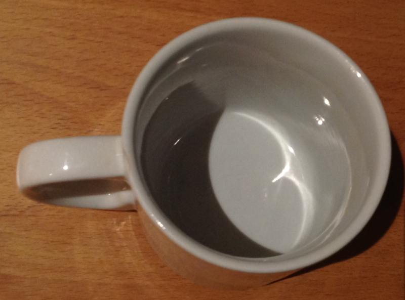
The reason for the formation of the catacaustic is that after the light is reflected on the inner wall of the cup, the distribution of photons is uneven, and some areas have a particularly high density of photons, resulting in higher brightness.
The catacaustic is a curve that is tangent to all reflected rays, meaning it is the envelope of all reflected rays. The specific shape of catacaustic depends on the shape of the cup and the position of the light source. Assuming the cup is circular, when the light source is a point source located exactly on the edge of the cup, the resulting catacaustic is a cardioid. When the light source is at infinity (can be considered as a parallel light source), the resulting catacaustic is a nephroid. In general, the shape of the catacaustic lies between a cardioid and a nephroid.
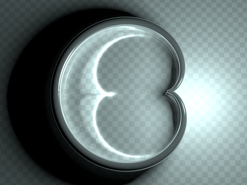
What’s even more interesting is that if the shape of the cup is the cardioid curve, and the light source is positioned exactly at the cusp. The resulting catacaustic is exactly the nephroid. I wrote a POV-Ray script to simulate this phenomenon.
| A cardioid catacaustic | A nephroid catacaustic |
 |
 |
It is worth noting that both the cardioid and the nephroid are so-called epicycloids, with the only difference being the ratio of the radii of the two circles.
| Cardioid | Nephroid |
It seems that we can make the following conjecture: if we place a light source inside or at the cusp of a nephroid, will we obtain another epicycloid? However, according to Greg Egan’s experiment on his blog, this should not hold true.
In theory, this POV-Ray script can render the effect of any parameter curve reflection (you need to make some modifications yourself, such as adjusting the scale and light source position). However, rendering parametric surface + radiosity in POV-Ray is very slow. So if you want to give it a try, it is best to use POV-Ray’s native CSG to construct the specular curve.
Catacaustics of parametric curves
In this section, we will introduce how to calculate the catacaustic of a general parameter curve \(\mathbf{c}(t)=(x(t),y(t))\)。
If the position of the light source is \((a,b)\), then at a point \((x,y)\) on the curve, the direction of the incident light ray is \[\mathbf{l}=(x-a,y-b).\] We don’t need to normalize \(\mathbf{l}\) because we will only need the direction of the light ray and not its length.
At the same point \((x,y)\), the normal vector of the curve is \[\mathbf{n}=\frac{(-y', x')}{\sqrt{(x')^2+(y')^2}}=\frac{(-y', x')}{|\mathbf{c}'|}.\]
so the direction of the reflected ray at point \((x,y)\) is given by the following reflection formula: \[\mathbf{r}= \mathbf{l}- 2(\mathbf{l}\cdot \mathbf{n})\mathbf{n}.\]
Let \((X,Y)\) be any point on the reflected ray, since \((x,y)\) is the starting point of the reflected ray, \((X-x,Y-y)\) is parallel to \(\mathbf{r}\). Let \(\mathbf{r}=(r_x,r_y)\), then \((X-x,Y-y)\) is perpendicular to \((-r_y, r_x)\), that is, \[(X-x, Y-y)\cdot(-r_y, r_x)=0.\] Let \[F(X,Y,t)=(X-x, Y-y)\cdot(-r_y, r_x),\] then we obtain the equation of the curve family satisfied by the reflected ray: \(F(X,Y,t)=0\). Therefore, the catacaustic, as the envelope of all reflected rays, can be obtained by solving the system of equations \[\begin{align*}F(X,Y,t)=0,\\\frac{\partial F}{\partial t}F(X,Y,t)=0.\end{align*}\] that is, \[\begin{align*}(X-x, Y-y)\cdot(-r_y, r_x)&=0,\\-(x',y')\cdot(-r_y, r_x) + (X-x,Y-y)\cdot(-r_y', r_x') &=0.\end{align*}\] And then solving for \(X,Y\).
If you still remember the inverse formula of a 2x2 matrix, the solution to this system of equations can actually be visually written out. Let’s rewrite it as
\[\begin{pmatrix}-r_y & r_x\\ -r_y'&r_x'\end{pmatrix}\cdot\begin{pmatrix}X-x\\Y-y\end{pmatrix}=\begin{pmatrix}0\\ r_xy'-r_yx'\end{pmatrix}.\] So \[\begin{align*}\begin{pmatrix}X-x\\Y-y\end{pmatrix}&=\begin{pmatrix}-r_y & r_x\\ -r_y'&r_x'\end{pmatrix}^{-1}\begin{pmatrix}0\\ r_xy'- r_yx'\end{pmatrix}\\ &=\frac{1}{r_xr_y'-r_yr_x'}\begin{pmatrix}r_x' & -r_x\\ r_y'&-r_y\end{pmatrix}\begin{pmatrix}0\\ r_xy'-r_yx'\end{pmatrix}\\ &=\frac{r_xy'-r_yx'}{r_yr_x'-r_xr_y'}\begin{pmatrix}r_x\\ r_y\end{pmatrix}.\end{align*}\] That is, \[\begin{pmatrix}X\\ Y\end{pmatrix}=\begin{pmatrix}x\\y\end{pmatrix} + \frac{r_xy'-r_yx'}{r_yr_x'-r_xr_y'}\begin{pmatrix}r_x\\ r_y\end{pmatrix}.\]
According to the deductions above, I wrote a small script to
calculate the catacaustic of a circle using sympy
(version=1.12). The center of the circle is at the origin with a radius
of 1, and the light source is at \((1,0)\).
1 | |
The result returned by sympy is:
1 | |
This is exactly the parametric representation of the cardioid:
\[\left\{\begin{align*}x(t)&=\frac{\cos(2t) + 2\cos(t)}{3},\\ y(t)&=\frac{\sin(2t) + 2\sin(t)}{3}.\end{align*}\right.\]
Using this parameter, we continue to calculate the catacaustic obtained when the light source is placed at the cusp of the cardioid, corresponding to point \((-\frac{1}{3},0)\) when \(t=\pi\):
1 | |
sympy quickly calculated the correct result:
1 | |
It’s not difficult to verify
\[\begin{align*}\frac{\sin(t)\sin(2t) + \cos(t)}{3}&=\frac{3\cos(t) - \cos(3t)}{6},\\ \frac{-\sin(t)\cos(2t) + \sin(t)}{3}&=\frac{3\sin(t) - \sin(3t)}{6}.\end{align*}\]
This is exactly the parametric form in the Wikipedia page when \(a\) is set to \(a=1/6\).
Catacaustics of polynomial curves
Usually, the equation of a curve is given in the form of an implicit function \(P(x,y)=0\), where \(P\) is a polynomial in two variables \(x\) and \(y\). Such curves are called plane algebraic curves. In this case, solving for the catacaustic requires the use of tools like Gröbner bases.
Let’s go back to the case of parametric equations. We have already seen that in this case, the catacaustic \((X,Y)\) has an explicit expression
\[\begin{pmatrix}X\\ Y\end{pmatrix}=\begin{pmatrix}x\\y\end{pmatrix} + \frac{r_xy'-r_yx'}{r_yr_x'-r_xr_y'}\begin{pmatrix}r_x\\ r_y\end{pmatrix}.\]
Where \(x,y,r_x,r_y\) are functions in one-variable \(t\),and their derivatives are also computable, so \((X,Y)\) can be computed.
However, in the case of implicit functions, we do not have an expression for \(x,y\) in terms of \(t\). But it’s okay, let’s assume that there is such a parameter expression and see what conclusions we can draw. Let \(x=x(t),y=y(t)\) be functions of some parameter \(t\), and differentiating both sides of \(P(x,y)=0\) with respect to \(t\) yields \[\frac{\partial P}{\partial t}=\frac{\partial P}{\partial x}x'(t) + \frac{\partial P}{\partial y}y'(t)=0.\] Let \(k=-\frac{\partial P}{\partial x}/\frac{\partial P}{\partial y}\), then \(y'(t)=kx'(t)\).
For the two components \((r_x,r_y)\) of the reflected light \(\mathbf{r}\), we also use chain rule to differentiate them separately. We have \[\begin{align*}\frac{\partial r_x}{\partial t}&=\frac{\partial r_x}{\partial x}x'(t) + \frac{\partial r_x}{\partial y}y'(t),\\ \frac{\partial r_y}{\partial t}&=\frac{\partial r_y}{\partial x}x'(t) + \frac{\partial r_y}{\partial y}y'(t).\end{align*}\] so we find that the ratio \[\begin{align*} \frac{r_xy'-r_yx'}{r_yr_x'-r_xr_y'}&=\frac{r_xk-r_y}{r_y(\frac{\partial r_x}{\partial x}+\frac{\partial r_x}{\partial y}k)-r_x(\frac{\partial r_y}{\partial x} + \frac{\partial r_y}{\partial y}k)}\\ &=-\frac{r_x\frac{\partial P}{\partial x}+r_y\frac{\partial P}{\partial y}}{r_y(\frac{\partial r_x}{\partial x}\frac{\partial P}{\partial y}-\frac{\partial r_x}{\partial y}\frac{\partial P}{\partial x})-r_x(\frac{\partial r_y}{\partial x}\frac{\partial P}{\partial y} - \frac{\partial r_y}{\partial y}\frac{\partial P}{\partial x})}.\end{align*}\] becomes a quantity that does not explicitly depend on \(t\), i.e., the variable \(t\) “cancels out”. Substituting this into the expression for catacaustic above, we obtain \[\begin{pmatrix}X\\ Y\end{pmatrix}=\begin{pmatrix}x\\y\end{pmatrix}-\frac{r_x\frac{\partial P}{\partial x}+r_y\frac{\partial P}{\partial y}}{r_y(\frac{\partial r_x}{\partial x}\frac{\partial P}{\partial y}-\frac{\partial r_x}{\partial y}\frac{\partial P}{\partial x})-r_x(\frac{\partial r_y}{\partial x}\frac{\partial P}{\partial y} - \frac{\partial r_y}{\partial y}\frac{\partial P}{\partial x})}\begin{pmatrix}r_x\\ r_y\end{pmatrix}.\] This equation can be further simplified: noting that the normal vector at point \((x,y)\) is given by \(\mathbf{n}=\frac{\nabla P}{|\nabla P|}\), where \(\nabla P=(\frac{\partial P}{\partial x},\frac{\partial P}{\partial y})\). From \[\mathbf{r}= \mathbf{l}- 2(\mathbf{l}\cdot \mathbf{n})\mathbf{n}\] We can derive \[\mathbf{r}\cdot \nabla P=-\mathbf{l}\cdot \nabla P.\] and thus \[\begin{pmatrix}X\\ Y\end{pmatrix}=\begin{pmatrix}x\\y\end{pmatrix}+\frac{\mathbf{l}\cdot\nabla P}{r_y(\frac{\partial r_x}{\partial x}\frac{\partial P}{\partial y}-\frac{\partial r_x}{\partial y}\frac{\partial P}{\partial x})-r_x(\frac{\partial r_y}{\partial x}\frac{\partial P}{\partial y} - \frac{\partial r_y}{\partial y}\frac{\partial P}{\partial x})}\begin{pmatrix}r_x\\ r_y\end{pmatrix}.\] These are two equations satisfied by four variables \((x,y,X,Y)\), in the form of \(F(X,x,y)=0\) and \(G(Y,x,y)=0\). Remember that we also have a known equation \(P(x,y)=0\). In order to eliminate \(x,y\) from these three equations and obtain an expression that only contains \((X,Y)\), we can try using the Gröbner basis method. The Gröbner basis method transforms the polynomial system
\[F=G=P=0\] into a set of equivalent new equations \[g_1=g_2=\cdots=g_m=0.\] which have exactly the same solution set.
\(\{g_1,\ldots,g_m\}\) is a set of generators of the ideal \(I=\langle F,G,P\rangle\) generated by \(F,G,P\) in the ring \(\mathbb{R}[x,y,X,Y]\), and \(\{g_1,\ldots,g_m\}\) is called the reduced Gröbner basis of \(I\). Under lexicographic order, the reduced Gröbner basis has a nice property that when changing from \(g_1\) to \(g_m\), the variables in the polynomials \(\{g_1,\ldots,g_m\}\) are eliminated in the order \(x\to y\to X\to Y\). Note that this is not a rigorous statement, as we cannot always eliminate variables in this order, but if elimination occurs, it will follow this order. This allows us to perform a “back-substitution” operation similar to the Gaussian elimination. As a result, solving the new system of equations will be simpler than the original one.
Let’s try an experiment with sympy:
1 | |
The last item of the given results is
\[27 X^{4} y^{2} + 54 X^{2} Y^{2} y^{2} - 18 X^{2} y^{2} - 8 X y^{2} + 27 Y^{4} y^{2} - 18 Y^{2} y^{2} - y^{2}.\]
\(x\) has been eliminated! The solutions to the original system of equations \(F=G=P\) must necessarily be a subset of the solutions to the above single equation. Observing each term, it is evident that they all contain a term \(y^2\), which is clearly not the solution we want. Removing it, we are left with the remaining factor
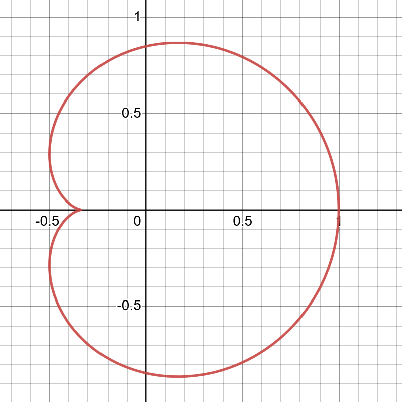
\[27X^{4}+54X^{2}Y^{2}-18X^{2} -8X + 27Y^{4}-18Y^{2}-1=0.\]
It is the implicit function representation of the cardioid. Don’t believe it? Let’s draw it in Desmos!
Some notes
This article mainly covers the first half of Greg Egan’s blog post. I feel that the second half is a bit too technical, so I decided not to cover it.
Although our experiment with sympy was very successful,
but keep in mind that it is not always possible to obtain the
catacaustic in all situations, and calculating curves with complicated
expressions in sympy can be very slow.
During my graduate studies, I took a course on computer algebra, and
at that time, we used Maple as the teaching software. Programming is
Maple was very inconvenient, so I actually don’t have much experience in
computer algebra programming. I used to think that sympy
was slow and the output were not simplified enough, so I was not very
willing to use it. This experiment has somewhat refreshed my
understanding of sympy. I still remember that the course
required each of us to submit a book report, and I wrote notes on
“Ideals, Varieties, and Algorithms”. But it’s been many years since
graduation, and this is the first time I’ve used Gröbner bases!