If you have heard of Lie algebras, chances are you have encountered the following pattern: (Refer to Wikipedia’s Lie algebra entry)

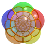
It displays the root system diagram for the Lie algebra \(E_8\), which consists of 240 vectors in an eight-dimensional Euclidean space \(\mathbb{R}^8\), each vector having exactly 56 nearest neighbors. Projecting these 240 vectors onto a special two-dimensional plane (known as the Coxeter plane) reveals a rotationally symmetric pattern, as seen in the figure above, where the 240 projected points are distributed across 8 concentric circles, each containing 30 evenly spaced vertices, thus remaining invariant under a rotation of angle \(\frac{2\pi}{30}\). The number \(h=30\) is called the Coxeter number of \(E_8\).

This phenomenon is not unique to \(E_8\) but holds for any finite Coxeter group, as illustrated by the following figure, which shows the pattern obtained by projecting the 32 vertices of a 5-dimensional hypercube and its edges onto its Coxeter plane:

Two vertices are projected to the origin, with the remaining 30 vertices distributed across 3 concentric circles, each containing 10 evenly spaced vertices. Hence the Coxeter number is \(h=10\).

In this blog post I will use \(E_8\) as an example to explain the mathematics behind this, following the presentation in section 3.16 of Humphreys’ textbook “Reflection Groups and Coxeter Groups”.

The code for this article is available on GitHub.

David Madore also has a beautiful interactive demo that can draw the root system of \(E_8\) in various ways.

The Structure of \(E_8\)

We know that the Dynkin diagram of \(E_8\) is as follows:

A set of simple roots is given by

\[\Delta=\begin{bmatrix}1&-1&0&0&0&0&0&0\\0&1&-1&0&0&0&0&0\\0&0&1&-1&0&0&0&0\\0&0&0&1&-1&0&0&0\\0&0&0&0&1&-1&0&0\\0&0&0&0&0&1&1&0\\-\frac{1}{2}&-\frac{1}{2}&-\frac{1}{2}&-\frac{1}{2}&-\frac{1}{2}&-\frac{1}{2}&-\frac{1}{2}&-\frac{1}{2}\\0&0&0&0&0&1&-1&0\end{bmatrix}.\]

Here, the vertex numbered \(i\) in the Dynkin diagram corresponds to the simple root \(\alpha_i\), which is the \(i\)th row of the matrix. Note that each simple root has a length of \(\sqrt{2}\), hence not a unit vector. This is mainly for convenience in later computations.

The Cartan matrix is given by

\[C=\left((\alpha_i,\alpha_j)\right)_{1\leq i,j\leq 8}=\begin{pmatrix}2&-1&0&0&0&0&0&0\\-1&2&-1&0&0&0&0&0\\0&-1&2&-1&0&0&0&0\\0&0&-1&2&-1&0&0&0\\0&0&0&-1&2&-1&0&-1\\0&0&0&0&-1&2&-1&0\\0&0&0&0&0&-1&2&0\\0&0&0&0&-1&0&0&2\end{pmatrix}.\]

Each simple root \(\alpha_i\) corresponds to a simple reflection \(s_i\):

\[s_i(v) = v - \frac{2(v,\alpha_i)}{(\alpha_i, \alpha_i)}\alpha_i = v-(v,\alpha_i)\alpha_i,\quad 1\leq i\leq 8.\]

Here, \((\,,\,)\) denotes the standard Euclidean inner product. This expression shows the advantage of making each simple root \(\alpha_i\) have a length of \(\sqrt{2}\): \(\alpha_i\) is equal to its coroot \(\frac{2\alpha_i}{(\alpha_i,\alpha_i)}\), resulting in the simple form of reflection about \(\alpha_i\).

To express this in code:

1
2
3
4
5
6
7
8
9
10
11
12
13
14
15
16

import numpy as np

# A set of simple roots listed by rows of 'delta'
delta = np.array([
    [1, -1, 0, 0, 0, 0, 0, 0],
    [0, 1, -1, 0, 0, 0, 0, 0],
    [0, 0, 1, -1, 0, 0, 0, 0],
    [0, 0, 0, 1, -1, 0, 0, 0],
    [0, 0, 0, 0, 1, -1, 0, 0],
    [0, 0, 0, 0, 0, 1, 1, 0],
    [-0.5, -0.5, -0.5, -0.5, -0.5, -0.5, -0.5, -0.5],
    [0, 0, 0, 0, 0, 1, -1, 0]
])

# The cartan matrix:
cartan = np.dot(delta, delta.transpose())

The group \(W\) generated by all simple reflections \(\{s_i\}\) is called the Weyl group of \(E_8\), containing 696729600 elements. The set \[\Phi = \{w\cdot\alpha\mid w\in W, \alpha\in\Delta\}\] generated by the action of the Weyl group on the simple roots is called the root system of \(E_8\), containing 240 distinct vectors, with \(W\) acting on \(\Phi\) by permutations.

The vectors in \(\Phi\) can be divided into two categories:

1. The first category includes all permutations of \((\pm1,\pm1,0,0,0,0,0,0)\), with two components being \(+1\) or \(-1\) and the remaining six being 0. There are 112 vectors of this type.
2. The second category includes vectors of the form \(1/2\times(\pm1,\pm1,\cdots,\pm1)\), where the number of \(-1\)s is even. There are 128 vectors of this type.

For programming convenience, we will multiply all roots by 2 to make them integer vectors. Thus, the code to generate the root system \(\Phi\) can be written as follows:

1
2
3
4
5
6
7
8
9
10
11
12
13
14
15
16
17
18
19
20
21
22
23
24
25
26
27

import itertools

roots = []

# Roots of the form (+-1, +-1, 0, 0, 0, 0, 0, 0),
# signs can be chosen independently and the two non-zeros can be anywhere.
for i, j in combinations(range(8), 2):
    for x, y in product([-2, 2], repeat=2):
        v = np.zeros(8)
        v[i] = x
        v[j] = y
        roots.append(v)

# Roots of the form 1/2 * (+-1, +-1, ..., +-1), signs can be chosen
# indenpendently except that there must be an even numer of -1s.
for v in product([-1, 1], repeat=8):
    if sum(v) % 4 == 0:
        roots.append(v)
roots = np.array(roots).astype(int)

# Connect a root to its nearest neighbors,
# two roots are connected if and only if they form an angle of pi/3.
edges = []
for i, r in enumerate(roots):
    for j, s in enumerate(roots[i + 1 :], i + 1):
        if np.sum((r - s) ** 2) == 8:
            edges.append([i, j])

Coxeter Element

Definition: An element \(\gamma\in W\) obtained by arranging the simple reflections \(s_1,\ldots,s_8\) in any order and then multiplying them is called a Coxeter element.

Coxeter elements are not unique but are all conjugate to each other ¹. Therefore, they share the same order, characteristic polynomial, and eigenvalues.

Definition: The order of any Coxeter element is called the Coxeter number of \(W\), denoted by \(h\).

Since \(\gamma\) is an element of the finite group \(W\), its 8 eigenvalues are of the form \[\{\zeta^{m_1},\ldots,\zeta^{m_8},0\leq m_i<h\}.\]

where \(\zeta\) is a primitive \(h\)-th root of unity. Section 3.16 in Humphrey’s boook shows that \(\gamma\)’s eigenvalues cannot be 1, so each \(1\leq m_i<h\). If \(\gamma\) has real eigenvalues, the only possibility is \(-1\) (corresponding to \(\zeta^{h/2}\)). \(\gamma\)’s complex eigenvalues appear in conjugate pairs, like \({\zeta^{m_i},\zeta^{h-m_i}}\).

A classical way to choose a Coxeter element is as follows: Note that the eight vertices of \(E_8\)’s Dynkin diagram can be divided into two groups, \(\{1, 3, 5, 7\}\) and \(\{2, 4, 6, 8\}\), with vertices within the same group not adjacent, hence the corresponding simple reflections commute. Let \[x=s_1s_3s_5s_7,\quad y=s_2s_4s_6s_8.\] Then \(\gamma=xy\) is a Coxeter element.

Coxeter Plane

Now let’s examine the Cartan matrix \(C\). We assert that \(C\) has an eigenvector \({\bf c}\) with all positive components and a multiplicity of 1. Note that the diagonal entries of \(C\) are all 2, and the off-diagonal entries are non-positive, making \(2I-C\) a non-negative matrix. Since \(E_8\) is an irreducible root system, both \(C\) and \(2I-C\) are irreducible matrices. By the Frobenius-Perron theorem, the largest eigenvalue of \(2I-C\) has a multiplicity of 1, and its corresponding eigenvector \({\bf c}\) has all positive components. \({\bf c}\) is naturally the smallest eigenvalue’s corresponding eigenvector of \(C\).

We can use numpy.linalg.eigh to find the eigenvalues and eigenvectors of the Cartan matrix \(C\):

1
2

eigenvals, eigenvecs = np.linalg.eigh(cartan)
c = eigenvecs[:, 0]

Where eigenvecs columns are all the eigenvectors of \(C\), arranged in ascending order of their eigenvalues. Therefore, the first column corresponds to the smallest eigenvalue’s eigenvector, which is our desired \({\bf c}\).

Following the notation on page 77 of Humphreys’ book:

Let \({\omega_i,1\leq i\leq 8}\) be the dual basis of \(\Delta\), i.e., \[(\alpha_i,\omega_j)=\delta_{ij}.\] Let \({\bf c}=(c_1,c_2,\ldots,c_8)\), and define \[\lambda = \sum_{i\in I}c_i\omega_i,\quad \mu= \sum_{j\in J}c_j\omega_j.\] Humphreys’ book shows that the two-dimensional plane \(P={\rm span}\{\lambda,\mu\}\) remains invariant under the actions of \(x,y\). In fact, \(x,y\) act as reflections on \(P\), thus \(\gamma=xy\) acts on \(P\) as a rotation. The order of this rotation is the order of \(\gamma\), which is the Coxeter number \(h\). Since \(\gamma\) permutes the root system \(\Phi\), projecting \(\Phi\) onto plane \(P\) theoretically should reveal a pattern with \(h\)-fold rotational symmetry. (In fact, this is the image at the beginning of this article)

Using the direct definitions of \(\lambda,\mu\) to compute the projection of \(\Phi\) onto \(P\) is inconvenient because it involves the dual basis \({\omega_i}\). We can bypass the calculation of the dual basis. This is implicitly suggested in the calculations on page 78 of Humphreys’ book:

If we define \[\nu=\sum_{j\in J}c_j\alpha_j.\] Then \(\mu=(1-c)\lambda+\nu\) and \(\nu\perp\lambda\). This amounts to say that \(\nu\) is the component of \(\mu\) perpendicular to \(\lambda\). Similarly, if we define \[\nu'=\sum_{i\in I}c_i\alpha_i.\] Then \(\nu'\) is the component of \(\lambda\) perpendicular to \(\mu\). Hence, \(P={\rm span}\{\nu,\nu'\}\). And \(\nu,\nu'\)’s expressions only involve \({\alpha_i}\), which simplifies the process.

The code can be written as follows (using \(u,v\) to represent \(\nu,\nu'\)):

1
2
3
4
5
6
7

I = [0, 2, 4, 6]
J = [1, 3, 5, 7]
u = sum(c[i] * delta[i] for i in I)
v = sum(c[j] * delta[j] for j in J)
u /= np.linalg.norm(u)
v -= np.dot(u, v) * u
v /= np.linalg.norm(v)

Here, we performed Gram-Schmidt orthogonalization on \(u,v\) to obtain an orthonormal basis for \(P\).

Projecting \(\Phi\) onto \(P\) is straightforward: for each vector in the root system, compute its coordinates in the basis \(u,v\):

1

roots_2d = [(np.dot(u, x), np.dot(v, x)) for x in roots]

What remains is to draw these points and the edges between them. The details of the drawing process are not discussed here.

Note: The inner product here is given by the Cartan matrix \(C\), and the orthogonalization and projection of the root system are also performed under this inner product. Since we represented \(u,v\) as combinations of the basis \(\Delta\), np.dot(x, u) actually computes the projection under the inner product defined by \(C\).

Further Improvement

If you look at the GitHub code, you’ll find that it’s not written exactly as described above. What’s the reason for this?

A minor drawback of the previous calculation is that we had to explicitly specify two sets \(I,J\). This step can also be avoided, but it requires a more detailed analysis of the Cartan matrix \(C\) and Coxeter element \(\gamma\). The following proposition can be found in Casselman’s article:

Proposition: \(2I + \gamma + \gamma^{-1}= (2I-C)^2\).

We can compute and verify that this identity indeed holds. Consider the matrix of \(\gamma\) under the basis \(\Delta\):

\[\gamma=xy=\begin{pmatrix}0&-1&1&0&0&0&0&0\\1&-1&1&0&0&0&0&0\\-1&1&-1&1&0&0&0&0\\0&0&1&-1&1&0&0&0\\0&0&1&-1&2&-1&1&-1\\0&0&0&0&1&-1&1&0\\0&0&0&0&1&-1&0&0\\0&0&0&0&1&0&0&-1\end{pmatrix}.\] Thus, \[\gamma^{-1} = yx=\begin{pmatrix}-1&1&0&0&0&0&0&0\\-1&1&-1&1&0&0&0&0\\0&1&-1&1&0&0&0&0\\0&1&-1&1&-1&1&0&1\\0&0&0&1&-1&1&0&1\\0&0&0&1&-1&1&-1&1\\0&0&0&0&0&1&-1&0\\0&0&0&1&-1&1&0&0\end{pmatrix}.\] Therefore, \[2I + \gamma + \gamma^{-1} = \begin{pmatrix} 1&0&1&0&0&0&0&0\\ 0&2&0&1&0&0&0&0\\ 1&0&2&0&1&0&0&0\\ 0&1&0&2&0&1&0&1\\ 0&0&1&0&3&0&1&0\\ 0&0&0&1&0&2&0&1\\ 0&0&0&0&1&0&1&0\\ 0&0&0&1&0&1&0&1 \end{pmatrix}=(2I - C)^2.\] This implies that \(v\) is an eigenvector of \((2I-C)^2\) with an eigenvalue of \(4\cos^2\frac{\theta}{2}\).

It seems to suggest that \(v\) is also an eigenvector of \(2I-C\) with eigenvalues of \(\pm 2\cos\frac{\theta}{2}\). However, it’s not clear whether both \(\pm 2\cos\frac{\theta}{2}\) will appear, or if they do, whether their multiplicities are equal.

Casselman demonstrated that this is indeed the case:

Proposition: \(2I-C\) and \(C-2I\) have the same characteristic polynomial.

According to this proposition, \(2I-C\) and \(C-2I\) have the same dimension for their eigenspaces corresponding to an eigenvalue \(\lambda\). Since the latter is the eigenspace of \(2I-C\) for the eigenvalue \(-\lambda\), it follows that the dimensions of the eigenspaces of \(C-2I\) for \(\pm\lambda\) are equal. Let \(V_s,V_{\bar{s}}\) be the eigenspaces corresponding to a pair of conjugate complex eigenvalues \(s=e^{i\theta}\) and \(\bar{s}=e^{-i\theta}\) of \(\gamma\). We have seen that \(P=V_s\oplus V_{\bar{s}}\) is the eigenspace of \((2I-C)^2\) for the eigenvalue \(4\cos^2\frac{\theta}{2}\). Since \(2I-C\) commutes with \((2I-C)^2\), \(P\) is also an invariant subspace of \(2I-C\). \(2I-C\) is diagonalizable on \(P\), making \(P\) the direct sum of eigenspaces of \(2I-C\) for eigenvalues \(\pm 2\cos\frac{\theta}{2}\). Thus, \(P\) is the direct sum of eigenspaces of \(C\) for eigenvalues \(2\pm2\cos\frac{\theta}{2}\).

Let’s verify this: the eigenvalues of \(C\) returned by numpy.linalg.eigh are as follows:

1

[0.01095621 0.51371035 1.18652671 1.58417662 2.41582338 2.81347329 3.48628965 3.98904379]

The sum of the first and the last is 4, the second and the second-to-last also sum to 4, the third and the third-to-last sum to 4, and the fourth and fifth sum to 4. Therefore, the eigenvalues of \(C\) sum pairwise to 4, consistent with the theory!

Generally, the dimension of \(P=V_s\oplus V_{\bar{s}}\) might not be 2, so \(P\) might not always be a plane. However, for the smallest eigenvalue of \(C\), we already know its multiplicity is 1, hence the multiplicity of its largest eigenvalue is also 1, making \(P\) a two-dimensional plane. Thus, \(\gamma\)’s action on \(P\) is a rotation of angle \(\theta_0\).

From the printed results, we see

\[0.01095621 \approx 2-2\cos\frac{\theta_0}{2},\quad \theta_0\approx 2\arccos0.994521895\approx\frac{2\pi}{30}.\] This verifies that \(\gamma\)’s action on \(P\) is a rotation of order 30, confirming the Coxeter number of \(W\) is 30.

To find a basis for \(P\), one needs only to find the eigenvectors \(u,v\) corresponding to the smallest and largest eigenvalues of \(C\), \[\alpha=\sum_{i=1}^8 u_i\alpha_i,\quad \beta=\sum_{i=1}^8 v_i\alpha_i.\] These form a basis for \(P\).