This program can help you make gif animations of various algorithms running on the 2d square grid.

Requirements: tqdm for showing process bar and pillow for reading images.

Examples

• Wilson's uniform spanning tree algorithm (my favourite, 2349 frames, 333KB, generated in 3 seconds):

  

• Prim's algorithm:

  

• Kruskal's algorithm:

  

• Langton's ant:

  

• Hilbert curve：

  

• Conway's game of life (gosper glider gun):

  

What's special about this program

The code is implemented in pure Python, no third-party modules nor softwares are required, just built-in modules like struct, random, colorsys and some built-in functions, and without any "color" or "draw" function calls. In later versions I added some features like showing process bars (requires tqdm) and enabling the user to embed the animtion into a background image (requires pillow). The program runs much faster than expected, it can generate highly optimized gif output in only a few seconds. One drawback is that it's not quite user-friendly: the user must have some basic knowledge of the GIF89a specification to know how to set parameters correctly in the animation.

How did this program come out

This program is motivated by Mike Bostock's wonderful Javascript animation. A few years ago when I saw Mike's page I immediately had the idea of writing a Python version to produce gif animations of Wilson's algorithm. A first thought on this was to save the animation into frames and then pack them back into a whole gif. But the animation usually contains thousands of frames so this is definitely a horrible task and is far from being efficient. Luckily five years later I learnt the GIF89a specification by chance and suddenly realized the new approach of encoding the animation into a byte stream. So basically I implemented a small gif encoder first, then run the algorithm on a 2d grid (use a 2d array to represent it) and encode it into frames along the way.

What is Wilson's algorithm

Consider the following problem:

Problem: Let \(G\) be a finite, connected and undirected graph. How can one choose a random spanning tree among all spanning trees of \(G\) from uniform probability? (we shall call such a tree an uniform spanning tree, or simply an UST.)

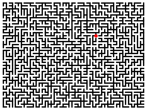
The following image shows an UST of a 48x36 grid, the circled dot is the root vertex:

You might say "that's easy, just write a program that lists all spanning trees and then use a random integer to choose one". But let's consider the complete graph \(K_n\) for example: \(K_n\) has \(n^{n/2}\) many different spanning trees by Cayley's formula, for \(n=100\) this number is \(100^{98}\), far more larger than the number of particles in the universe! (which is estimated about \(10^{90}\))

Currently the most efficient algorithm known is the one proposed in Wilson's paper

"generating random spanning trees more quickly than the cover time".

It's a random algorithm, that is, some times you may be very lucky to get an UST soon, or you may wait forever. But one can prove that this algorithm will terminate in finite steps with probability one (note this does not exclude the possibility of running forever, think about this), and it performs really well in most cases.

The key to understand Wilson's algorithm is the so called loop erased random walk, that is, once the random walk visits a vertex that already existed in its path, it immediately erases the loop between these two visits and continues the walk from this vertex. Just watch the Javascript animation if you don't understand this, it's obvious to see what "loop erased random walk" means from it. (click on the canvas to restart the animation)

The algorithm runs as follows:

Wilson's algorithm:

1. Choose any vertex \(v\) as the root and maintain a tree \(T\), initially \(T=\{v\}\).
2. For any vertex \(z\) that is not in \(T\), start a loop erased random walk from \(z\) until the walk hits \(T\), then add the resulting path of the walk to \(T\).
3. Repeat step 2 until all vertices of the graph are in \(T\).

The proof of the correctness of this algorithm is a bit tricky and will not be discussed here, you may refer to Wilson's original paper or the book by Russell Lyons and Yuval Peres:

"Probability on Trees and Networks".

Implementation

As mentioned before, the animation of Wilson's algorithm (and also Langton's ant animation) usually contains thousands of frames in it, so it's quite surprising that this program takes only a few seconds to produce a highly optimized image. The key points are:

• Only encode a minimum region at a time. We can maintain a rectangular region to store which cells are changed between successive frames, this enables us to encode only a small portion of the window instead of the whole into a frame.

• Use variable mimimum code length for the LZW compression. When encoding a frame into bytearrays LZW compression allows the minimum code length \(k\) can be as small as the color depth of this frame (and must satisfy \(2\leq k\leq12\)), this is another benifit since most frames only contain very few colors.

• Write the frames to a temporary BytesIO file in memory and flush it to disk in the end.

The code is divided into three layers: at the top layer is the Maze class on which we run various algoirthms. This layer knows nothing about the gif image. At the bottom layer is the GIFSurface class which holds the raw information like image size, global color table, number of loops, background color index, etc. It knows nothing about the Maze. At the middle layer is the Animation class which controls how the Maze is encoded and writes to the GIFSurface.

A short introduction to the GIF89a specification

In this section I'll give a not-so-detailed introduction to the GIF89a specification. It's not meant to be comprehensive nor self-contained, you should always refer to What's in a GIF when you have difficulties understanding my words here.

Roughly a GIF image consists of:

Structure of a GIF File

1. Always begins with 6 bytes GIF89a.
2. Then follows the logical screen descriptor which specifies the width and height of the image and the size of the global color table.
3. Then follows the global color table.
4. Then follows the loop control block which specifies the number of loops of the image.
5. Then comes the actual data of the frames. The data of each frame can be further divided into 3 parts:
   1. the graphics control block which specifies the delay and transparent color of this frame.
   2. the image descriptor which specifies the relative position of this frame in the window and the size of the local color table.
   3. the local color table of this frame (if there is a local color table for this frame).
   4. the LZW compressed pixel data of this frame.
6. Finally the image file ends with a byte 0x3B.

Note: the above description does not apply to all GIF images, there can be some variations. For example:

1. The image may not contain a global color table (so you have to specify a local color table for each frame).

2. For a static image the loop control block is not required; for a stacit frame the graphcs control block is not required.

3. The file may end without the byte 0x3B, most decoders can still decode the image correctly.

Now we explain each part in more details.

The header GIF89a

In python you can write it as

1

struct.pack('6s', b'GIF89a')

Why b'GIF89a' not simply 'GIF89a'? This is for compatibility with Python2 and 3 since the default encoding in Python3 is unicode whereas in python2 it's ascii.

The logical screen descriptor

Example:

1

struct.pack('<2H3B', width, height, 0b10010001, 0, 0)

Here you shoud note the format string < (little endian).

The byte 0b10010001 is called a packed field. Let's read it from left to right:

1. The first bit 1 means we have a global color table (0 for absent).
2. The next 3 bits specify the "color depth". You don't need care about what they mean since modern decoders like firefox and chrome do not use them.
3. The fifth bit is the "sort flag" and is not used today, always set to 0.
4. The ending 3 bits represent an integer \(x\) in range 0-7, \(x\) specifies the size of the global color table (\(=2^{x+1})\).

The last two bytes are of little importance and we don't discuss them here.

Global color table

Example: if we want to use 4 colors red, green, blue, yellow, then the global color table can be written as

1

bytearray([255, 0, 0, 0, 255, 0, 0, 0, 255, 255, 255, 0])

It's important that the number of colors in this array must be a power of 2 and match the size of the global color table specified in the packed byte in the logical screen descriptor, otherwise the decoder will not be able to parse the image correctly.

Graphics control block

Example:

1

struct.pack("<4BH2B", 0x21, 0xF9, 4, 0b00000101, delay, trans_index, 0)

The 3 beginning bytes 0x21, 0xF9, 4 are fixed and are used to inform the decoder "Hey, I'm a graphics control block, see the next 4 bytes!"

The next byte 0b00000101 is also a packed field, let's read it from left to right:

1. The first 3 bits are useless and are always 0.
2. The next 3 bits are called "desposal method", they represent an integer \(x\) in range 0-7 and \(x\) specifies how we should dispose this frame after it's displayed.

   1. \(x=0\) means it's undefined, decoders will use default 1 instead in this case.

   2. \(x=1\) is the default, it means leave this frame here. So if the next frame is not overlapped with this frame then both these two frames will be displayed. Otherwise the overlapped area in this frame will be covered by the next one. See the example below:

      

   3. \(x=2\) means remove this frame and restore the image to background image/color, see the following example:

      

      You can see each frame is remove immediately after it's displayed, and its region is filled with transparent background (so you are really seeing the browser's background color through the image).

   4. \(x=3\) also means remove this frame, but restore the image to the previous frame.

   5. 4-7 are unused.

The next 2 bytes delay specifies the delay of the frame in centiseconds, so delay=3 means "keep staying here for 0.03 second".

The last byte trans_index specifies the transparent color in this frame, the pixels in this frame using this color are transparent: you can see the previous frame through them (of course only when the previous frame is still there (reserved), otherwise you are seeing the previous previous frame, ..., etc).

Image descriptor block

Example:

1

struct.pack('<B4HB', 0x2C, left, top, width, height, 0)

Quite straight-forward to understand. Note the last byte is 0 since we do not need local color tables here.

The LZW compression algorithm

Finally we are left with the most difficult part: the LZW algorithm. It's too long to include an introduction to the algorithm here, so please refer to the second article in What's in a gif for a complete treatment. But it's quite simple to implement it in Python, see the file encoder.py for an example.