Coxeter groups, automata and uniform tilings
Since using POV-Ray to render 3D hyperbolic honeycombs was incredibly slow, I’ve decided to abandon this approach and have removed the code from the main branch on GitHub. You can find the code used in this article in the old release version. For how to render hyperbolic honeycombs, readers can refer to another project.
This article introduces a Python program I just finished. Although it’s freshly completed, it took up most of my free time over the last six months. It was quite the challenge, requiring a lot of effort and dedication. The main reason is that it involves a few complicated theories, specifically the deep properties of Coxeter groups, known as the automatic property. A significant portion of these months was spent learning from articles by Casselman, Brink & Howlett, and others, which helped me understand the mathematicas of this project (see references at the end).
Although finishing this program is a great achievement for me, I don’t mean to boast about any superiority of this program: the computational method it uses for Coxeter groups is not advanced and might not impress the experts. Moreover, its code is somewhat ugly, and likely difficult for other people to use.
The purpose of this program is to use group theory to draw various two-dimensional and three-dimensional uniform tilings. You can think of uniform tiling as using some regular polygons to tile the space so that the vertices of the tiles are transitive under the action of a symmetry group (forming a single orbit).
I will first show some examples of what this program can do, and then explain how it works.
Examples
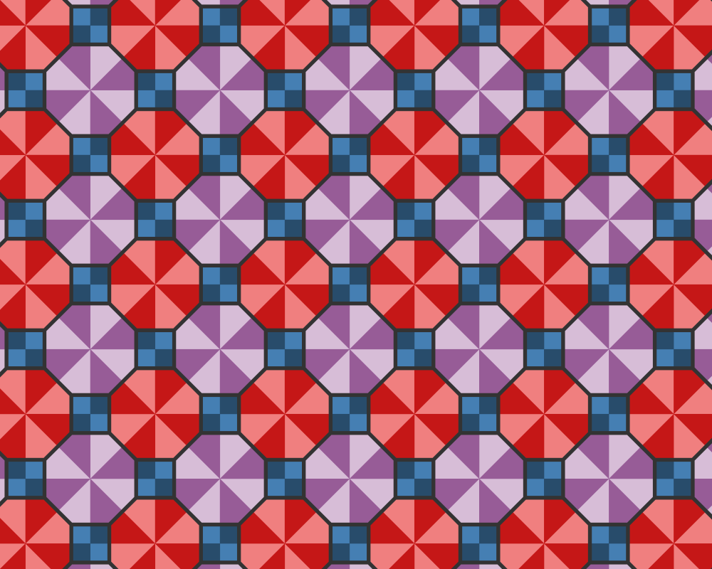
Below is the 2d Euclidean tiling omnitruncated (4, 2, 4):
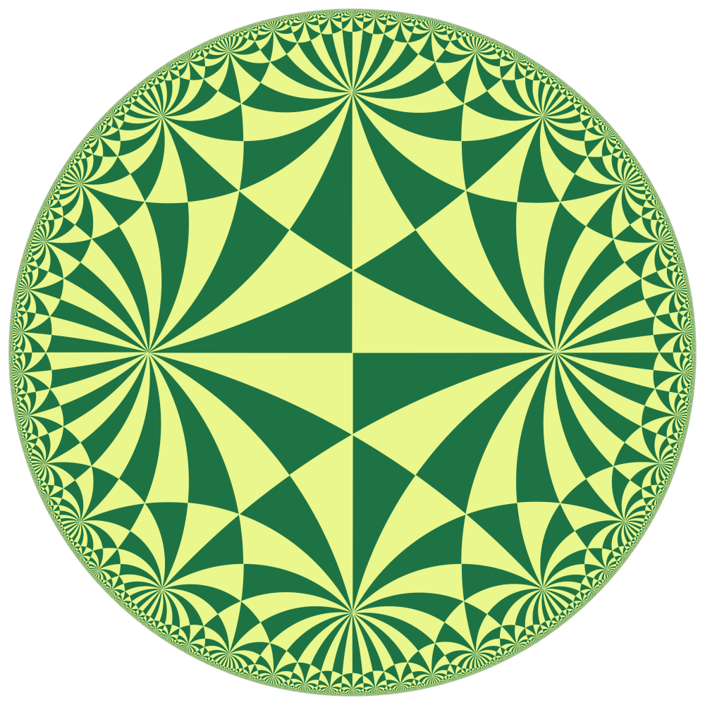
Below is the 2d hyperbolic tiling regular (2, 3, 13) in Poincaré’s disk model:
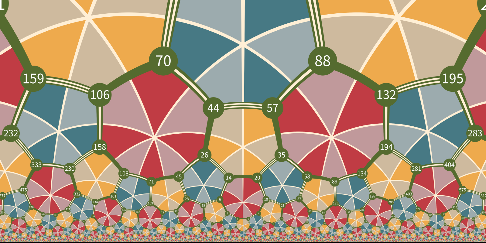
Below is the 2d hyperbolic tiling omnitruncated (4, 3, 3) in upper half plane model:
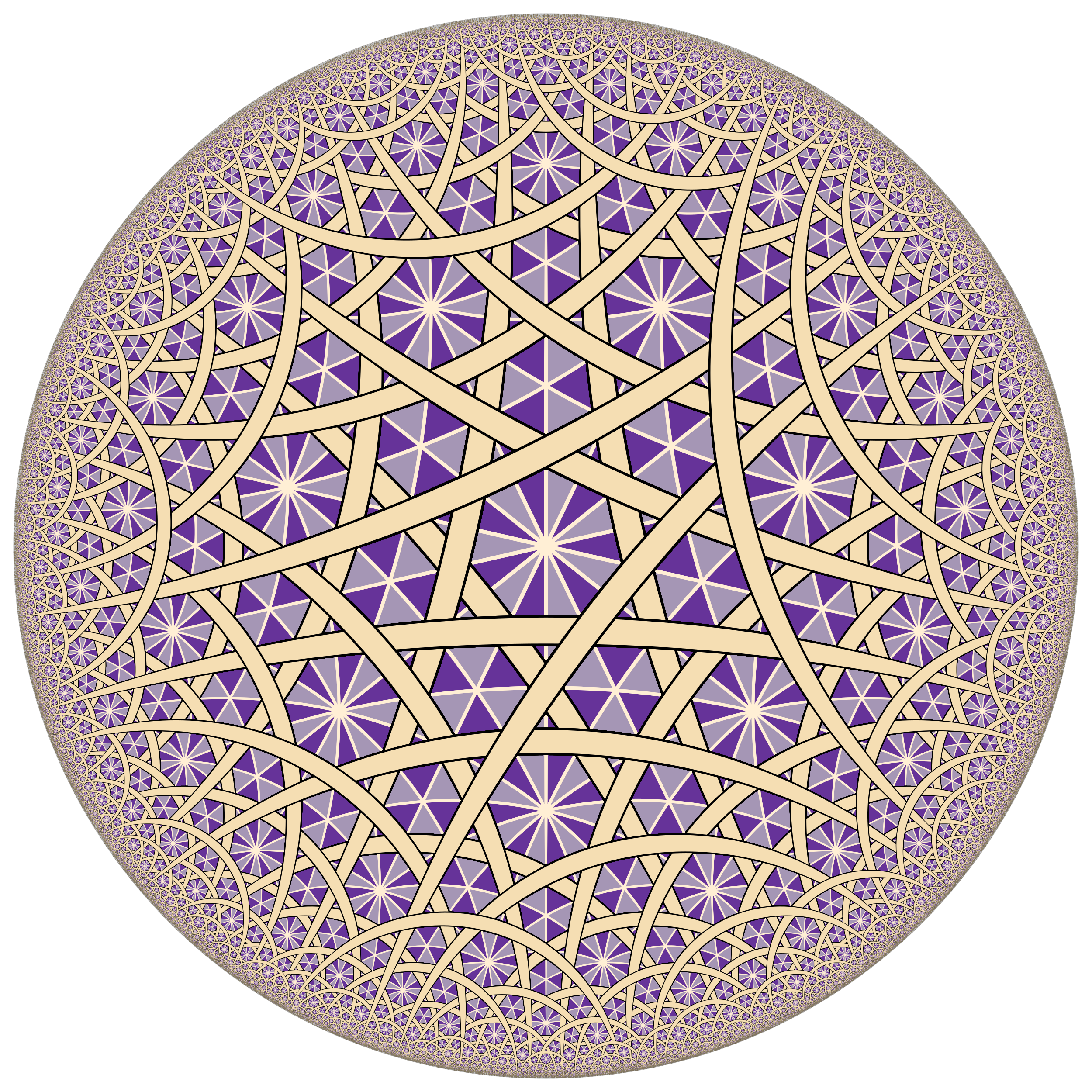
A hyperbolic weave pattern:
Below is the 3d hyperbolic tiling regular (3, 5, 3) in Poincaré’s ball model:
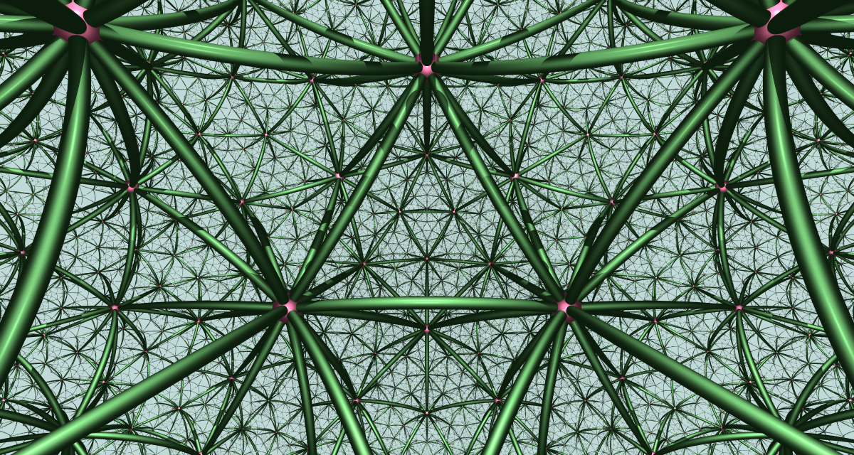
Below is the 3d hyperbolic tiling regular (5, 3, 5) in Poincaré’s ball model:
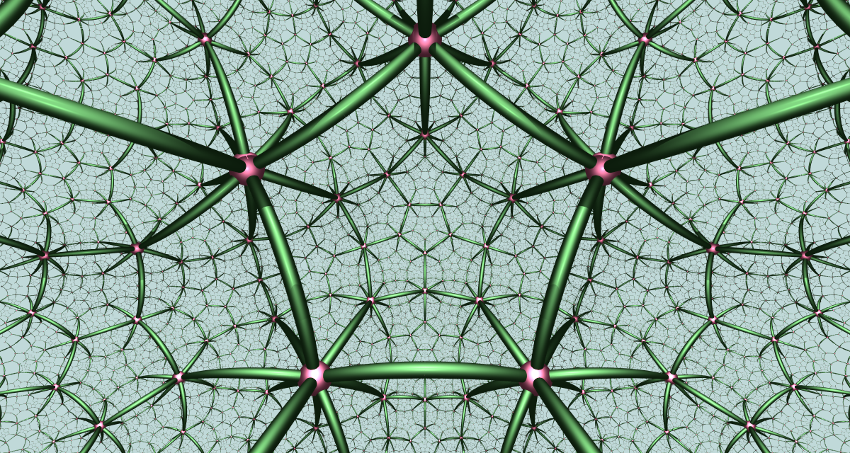
Below is the 3d hyperbolic tiling regular (5, 3, 4) in Poincaré’s ball model:
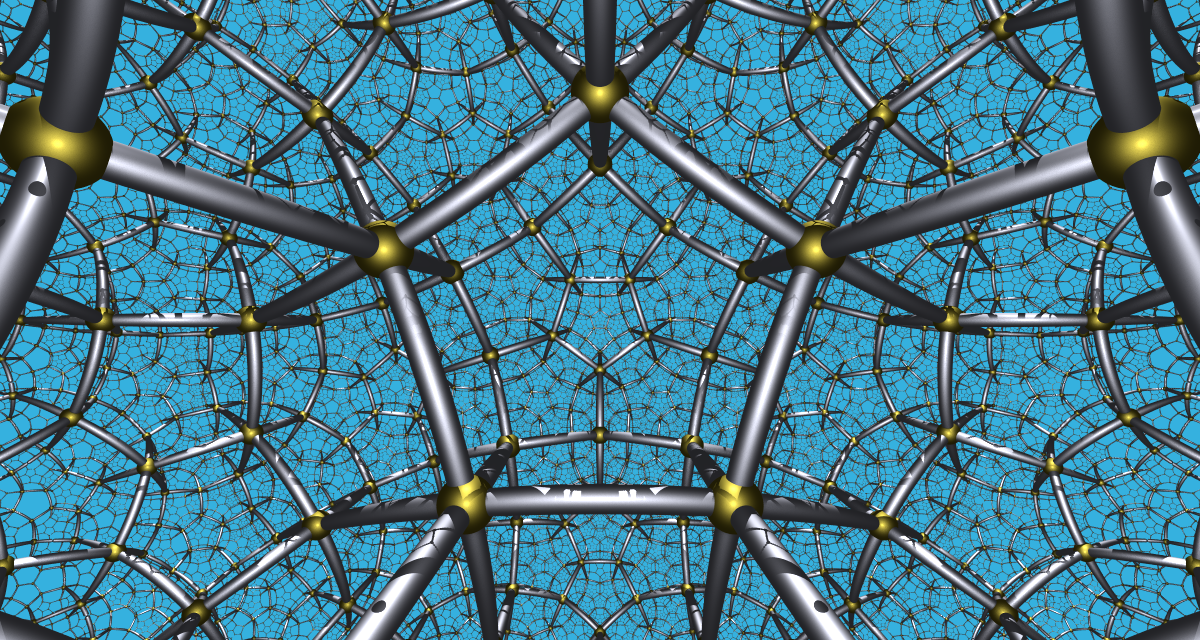
Below is the 3d hyperbolic tiling regular (4, 3, 5) in Poincaré’s ball model:
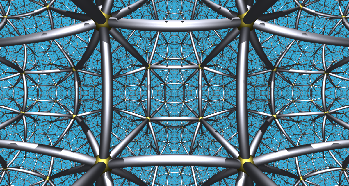
The above four regular tilings are the only regular ones with compact cells. If we drop the restriction on compactness and requires the cells must have finite volume, then we have ten more regular tilings, with each has a Euclidean vertex configure. For example (6, 3, 3):
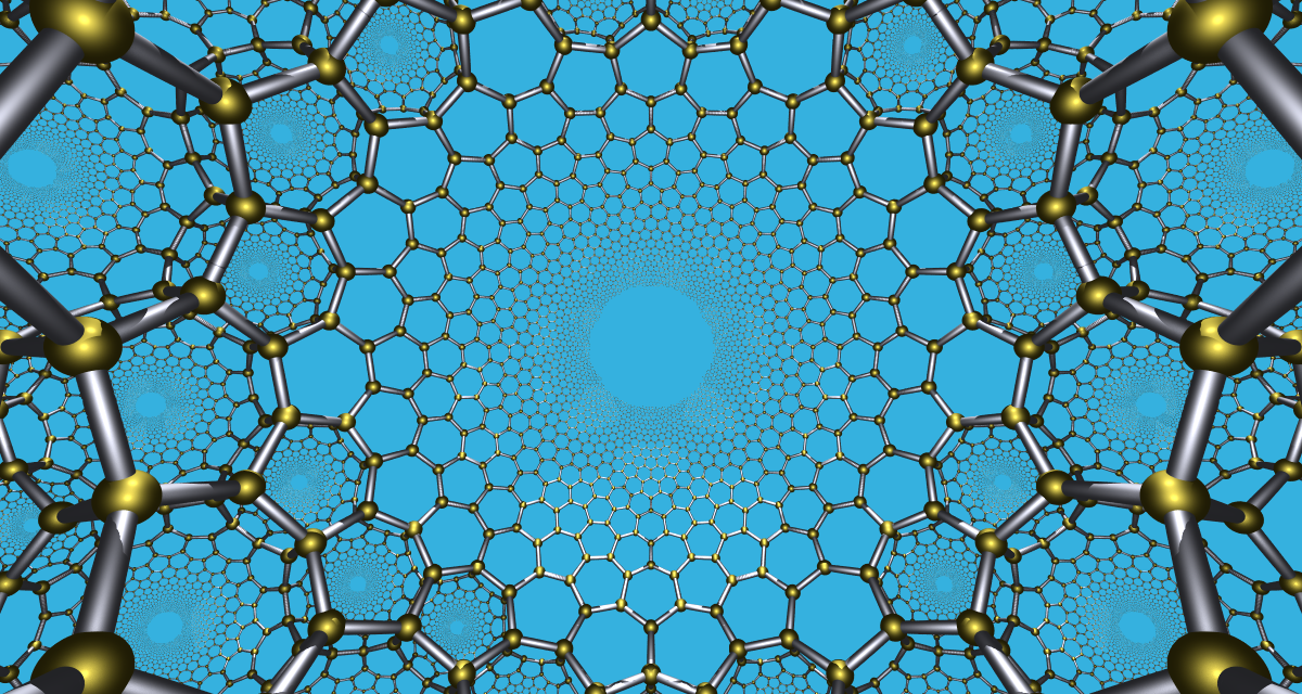
You can see the cells have ideal vertices, i.e. vertices at the infinity. These tilings are called “paracompact”.
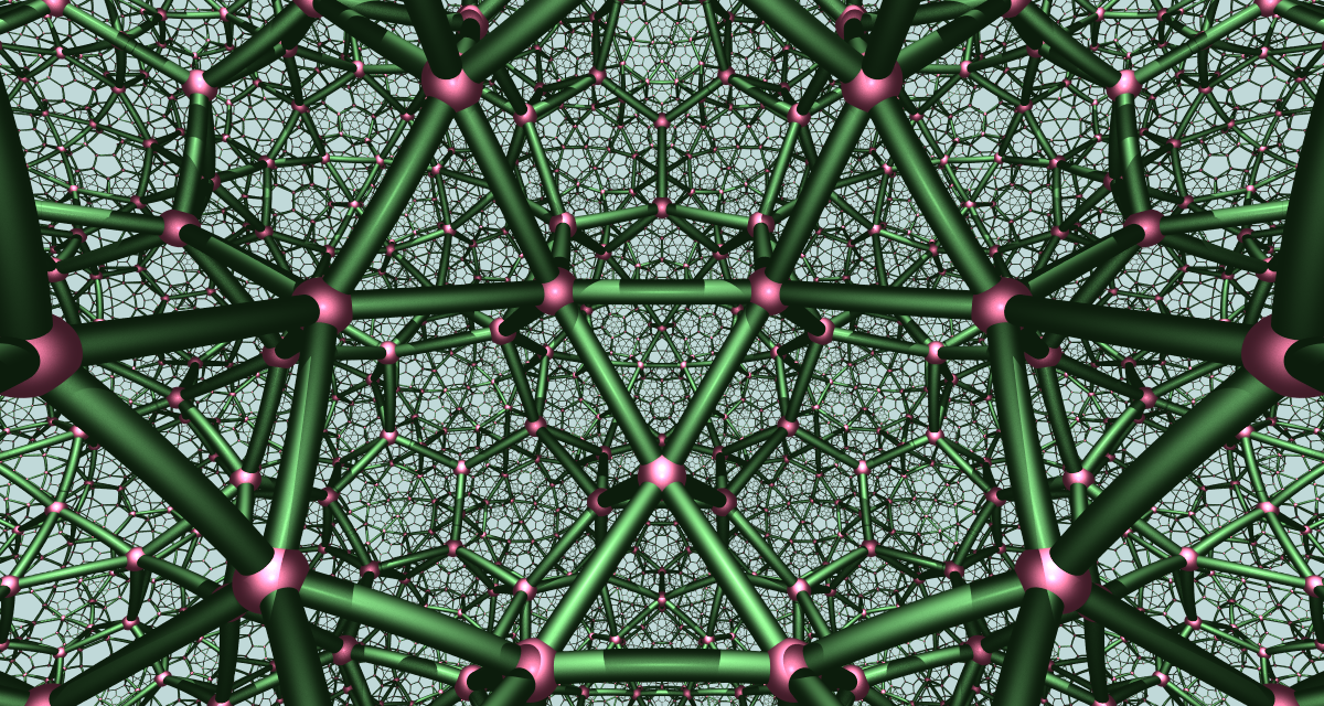
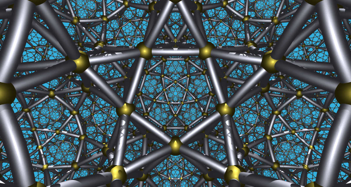
If we drop the restriction on being “regular” then we have lots more examples, like rectified (3, 5, 3) and rectified (5, 3, 4):
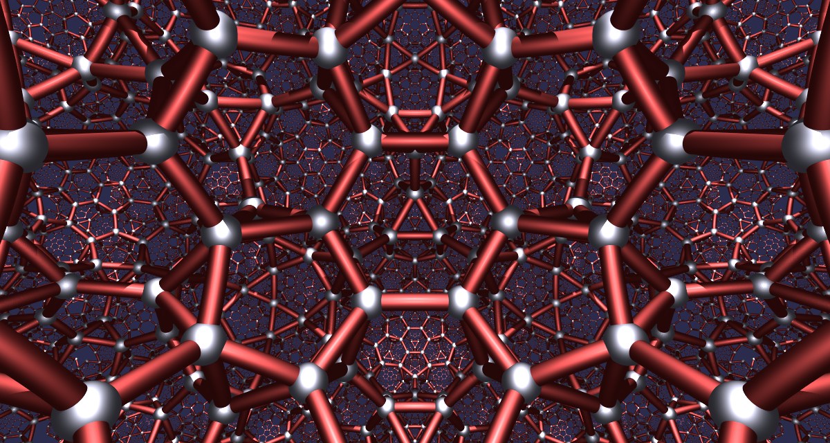
and the cantic order-5 cubic tiling from the [5, 31,1] family:
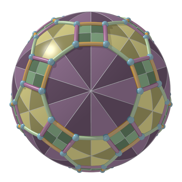
Below is a 2d spherical tiling rendered in 3d:
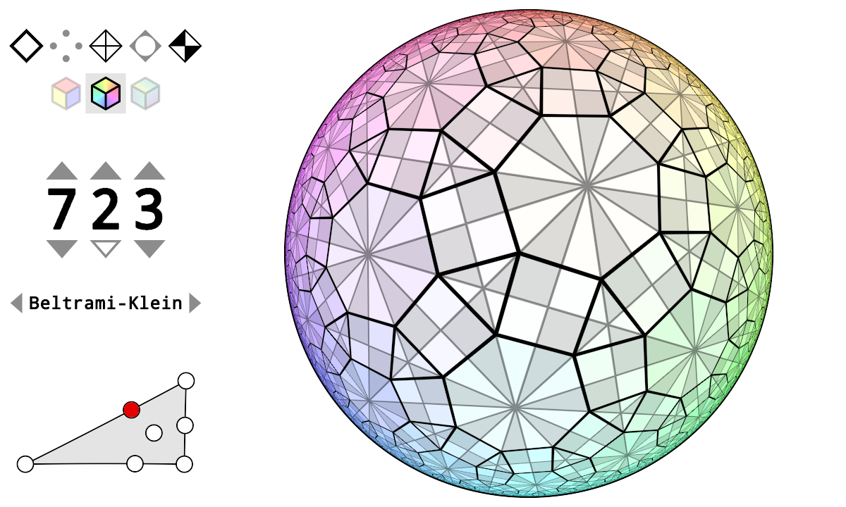
Finally a shader program exported from Matt Zucker’s excellent work on shadertoy:
Wythoff construction
The main theoretical tool for drawing uniform tilings is the so-called Wythoff construction, also known as the kaleidoscope method. This involves placing several reflecting planes (mirrors) in space, then starting from an initial point, and repeatedly applying reflection transformations about these mirrors to obtain all the virtual images, which gives all the vertices of the tiling.
The following video demonstrates the effect of the Wythoff construction: in the 2D Poincaré hyperbolic disk, the walls around the room are all mirrors. The scene in the room is repeatedly reflected in the mirrors, creating infinitely many virtual image rooms, filling the entire hyperbolic space. Note that, there is only one ‘real’ room, namely the room where the observer is standing in; all other rooms are virtual images of the real one.
There are two different approaches to implemente the Wythoff construction in a program:
Inverse Pixel Method. This method involves calculating, for each pixel in the image, its corresponding point \(p\) in the world space. Then, \(p\) is repeatedly reflected off mirrors until it falls within the fundamental region, say the final location is \(q\). Essentially, we find the pre-image \(q\) of \(p\) in the real room (called the fundamental domain). Then, based on \(q\)’s position within the fundamental domain, the pixel corresponding to \(p\) is colored. This method allows for parallel computation on all pixels, and when combined with shader programming, it can produce very stunning effects. Here are two examples from shadertoy:
The inverse pixel method cares solely about the final pixel color. It doesn’t care about the actual coordinates. It produces raster images and cannot output vector graphics. Moreover, exporting data for use in modeling software is not very convenient with this method.
Coordinate Method. This approach starts from a given initial point \(v_0\) and calculates all its virtual images (within some maximum number of vertices) as well as the connections between edges and faces, then draws them one by one. This method allows for the acquisition of specific vertex coordinate information and outputs vector graphics and model files, making it more suitable for usage in academic papers. However, it cannot be parallelized and is quite slow in computing hyperbolic tilings, as the structures grows exponentially.
My program uses the coordinate method. It first performs symbolic calculations within the symmetry group of the tiling to determine the word representation corresponding to each vertex in the shortest lexicographical order (a word is a tuple where each element is an integer), as well as the connections between edges and faces (also tuples of integers), and then applies the word corresponding to each vertex to the initial vertex to obtain the floating-point coordinates of that vertex. In other words, before computing the final coordinates of each vertex, it has already pre-calculated how many vertices there are, how each vertex is obtained through reflections from the initial vertex, which vertices form edges, which form faces, which form cells, etc. These calculations involve only integer operations, completely avoiding issues with floating-point precision loss.
Sounds amazing? Let me demonstrate the specific steps with an example.
Example: omnitruncated (7, 2, 3) tiling
The Coxeter-Dynkin diagram for the omnitruncated (7, 2, 3) tiling is:
This is a hyperbolic tiling, its symmetry group \(G\) is the Coxeter group determined by Coxeter matrix
\[M=\begin{pmatrix} 1 & 7 & 2 \\ 7 &1 &3\\ 2 & 3 &1\end{pmatrix}\]
and has presentation
\[W = \langle s_0,s_1, s_2\ |\ s_0^2=s_1^2=s_2^2=(s_0s_1)^7=(s_1s_2)^3=(s_0s_2)^2=1\rangle.\]
The initial vertex \(v_0\) is not on any of the three mirrors, so its stabilizing subgroup is \(\langle 1\rangle\), by orbit-stabilizer theorem each element \(w\) of \(W\) maps \(v_0\) to a distinct vertex in the tiling.
Every element \(w\) in \(W\) can be expressed as a product of the generators \(s_0,s_1,s_2\). We call any such expression a word representation of \(w\). If \(w=s_{i_1}s_{i_2}\cdots s_{i_k}\) is a word expression, and there are no other expressions of \(w\) with length less than \(k\), we call \(s_{i_1}s_{i_2}\cdots s_{i_k}\) a reduced expression, and define \(l(w)=k\) to be the length of \(w\). The reduced expression of \(w\) is generally not unique. For example, from the defining relations of \(W\), we can see that \(s_0s_2=s_2s_0\) and \(s_1s_2s_1=s_2s_1s_2\), etc. However, all reduced expressions of \(w\) must have the same length, so the definition of \(l(w)\) is reasonable.
We can choose a smallest one among all reduced expressions \(w\) as the normal form of \(w\). This sorting is called shortlex order. As the name implies, shortlex order is the order used by dictionaries to arrange words.
First, define the alphabetical order of the generators \(s_0,s_1,s_2\) as \(s_0<s_1<s_2\), then extend this order to any two reduced expression \(w_1\) and \(w_2\):
Shortlex Order: Let \(w_1 = s_{i_1}s_{i_2}\ldots s_{i_n}\) and \(w_2=s_{j_1}s_{j_2}\cdots s_{j_m}\) be two different reduced expressions, where \(w_1, w_2\) can be different group elements. The relationship between them in shortlex order is determined as follows:
- First, compare the lengths. If the lengths are different, the one with the shorter length is considered smaller, that is, if \(n < m\) then \(w_1 < w_2\), conversely if \(n > m\) then \(w_1 > w_2\).
- If the lengths are the same, then compare the alphabetical order from left to right. Let \(k\) be the first index such that for any \(l < k\), \(s_{i_l} = s_{j_l}\) but \(s_{i_k} \ne s_{j_k}\), then the relationship between \(w_1, w_2\) is the same as the relationship between \(s_{i_k}\) and \(s_{j_k}\).
Thus, every \(w\in W\) has a unique normal form under shortlex order.
Define \(\mathcal{SL}(W)\) as the set consisting of the normal forms of all elements in \(W\). Below is a list of all elements in \(\mathcal{SL}(W)\) with lengths up to 5, totaling 37: (arranged in rows from smallest to largest)
\[ \begin{array}{lllll}e&s_{0}&s_{1}&s_{2}&s_{0}s_{1}\\s_{0}s_{2}&s_{1}s_{0}&s_{1}s_{2}&s_{2}s_{1}&s_{0}s_{1}s_{0}\\s_{0}s_{1}s_{2}&s_{0}s_{2}s_{1}&s_{1}s_{0}s_{1}&s_{1}s_{0}s_{2}&s_{1}s_{2}s_{1}\\s_{2}s_{1}s_{0}&s_{0}s_{1}s_{0}s_{1}&s_{0}s_{1}s_{0}s_{2}&s_{0}s_{1}s_{2}s_{1}&s_{0}s_{2}s_{1}s_{0}\\s_{1}s_{0}s_{1}s_{0}&s_{1}s_{0}s_{1}s_{2}&s_{1}s_{0}s_{2}s_{1}&s_{1}s_{2}s_{1}s_{0}&s_{2}s_{1}s_{0}s_{1}\\s_{0}s_{1}s_{0}s_{1}s_{0}&s_{0}s_{1}s_{0}s_{1}s_{2}&s_{0}s_{1}s_{0}s_{2}s_{1}&s_{0}s_{1}s_{2}s_{1}s_{0}&s_{0}s_{2}s_{1}s_{0}s_{1}\\s_{1}s_{0}s_{1}s_{0}s_{1}&s_{1}s_{0}s_{1}s_{0}s_{2}&s_{1}s_{0}s_{1}s_{2}s_{1}&s_{1}s_{0}s_{2}s_{1}s_{0}&s_{1}s_{2}s_{1}s_{0}s_{1}\\s_{2}s_{1}s_{0}s_{1}s_{0}&s_{2}s_{1}s_{0}s_{1}s_{2}&\end{array} \]
Note the number of all words in \(s_0,s_1,s_2\) with length less or equal than five is \(1+3+\cdots+3^5=364\), the list above tells us that they indeed contain only 37 different ones, the remaining 364 - 37 = 327 ones are duplicates. A further computation shows that the number of all words with length no more than six is 1093 but they contain only 53 different elements. So we can gain a great improvement in efficiency if we only use words in \(\mathcal{SL}(W)\) instead of traversing all possible combinations of the generators.
How can we generate those words that are precisely in \(\mathcal{SL}(W)\)? This leads us to a very important theorem on Coxeter groups:
Theorem [Brigitte Brink & Robert B. Howlett, 1993]: If \(G\) is a finitely generated Coxeter group then \(\mathcal{SL}(W)\) is a regular language.
The term “regular language” comes from computer science, a basic fact about a regular language over a finite alphabetical set is that this language can always be recognized by a definite finite automaton (DFA), such DFA may not be unique but there is a “minimal one” with the least number of states and this minimal one is unique if we don’t distinct relabellings of the states.
Below is the automaton recognizes \(\mathcal{SL}(W)\) for the (7, 2, 3) group:
You can see there are 19 nodes (i.e. states) in the automaton. The labels of the states are irrevalent because renumbering the states of an automaton does not change the language it recognizes.
The red node is the initial state.
The directed edges in the graph tell us the transition rule between the states. The edges are labelled by the generators of the group, i.e. \(i\) for \(s_i\). If we start from the initial state and keep on moving to a next state along an edge up to a finite number of steps, then the path we travelled gives a word in \(\mathcal{SL}(W)\). All words in \(\mathcal{SL}(W)\) can be generated in this way.
For example:
- The only path of length 0 correspondes to the identidy 1.
- The three paths of length 1 \[\begin{align*} 0&\xrightarrow{\ s_0\ }1,\\ 0&\xrightarrow{\ s_1\ }2,\\ 0&\xrightarrow{\ s_2\ }8. \end{align*}\] corresponde to the three generators \(s_0,s_1,s_2\) in \(\mathcal{SL}(W)\).
- The five paths \[\begin{align*}0&\xrightarrow{\ s_0\ }1\xrightarrow{\ s_1\ }2\\ 0&\xrightarrow{\ s_0\ }1\xrightarrow{\ s_2\ }8\\ 0&\xrightarrow{\ s_1\ }2\xrightarrow{\ s_0\ }3\\ 0&\xrightarrow{\ s_1\ }2\xrightarrow{\ s_2\ }8\\ 0&\xrightarrow{\ s_2\ }8\xrightarrow{\ s_1\ }9\end{align*} \] corresponde to the five elements of length 2 in \(\mathcal{SL}(W)\): \(s_0s_1,s_0s_2,s_1s_0,s_1s_2,s_2s_1\).
Using breadth-first search we can easily generate all words in \(\mathcal{SL}(W)\) up to any given depth.
Note for an infinite Coxeter group the automaton must have cycles, but for a finite Coxeter group the automaton must be a directed tree, for example the symmetry group \(S_4\) of tetrahedron:
The 24 different paths corresponde to the 24 group elements of \(S_4\):
\[ \begin{array}{llll}e&s_{0}&s_{1}&s_{2}\\s_{0}s_{1}&s_{0}s_{2}&s_{1}s_{0}&s_{1}s_{2}\\s_{2}s_{1}&s_{0}s_{1}s_{0}&s_{0}s_{1}s_{2}&s_{0}s_{2}s_{1}\\s_{1}s_{0}s_{2}&s_{1}s_{2}s_{1}&s_{2}s_{1}s_{0}&s_{0}s_{1}s_{0}s_{2}\\s_{0}s_{1}s_{2}s_{1}&s_{0}s_{2}s_{1}s_{0}&s_{1}s_{0}s_{2}s_{1}&s_{1}s_{2}s_{1}s_{0}\\s_{0}s_{1}s_{0}s_{2}s_{1}&s_{0}s_{1}s_{2}s_{1}s_{0}&s_{1}s_{0}s_{2}s_{1}s_{0}&s_{0}s_{1}s_{0}s_{2}s_{1}s_{0}\end{array} \]
Now the big question:
Question 1: How to compute \(\mathcal{SL}(W)\)?
The answer to this question is too complicated to be covered in this article, a simple sketch of the main thread is appended at the end. When I was developing this program I mainly referred to Casselman’s notes 1 2 3 and the textbook by Humphreys 4. These should be enough for a reader with a solid background in undergradute abstract algebra.
Once we have the normal forms of the group elements, we can easily use them to map the initial vertex \(v_0\) to other vertices in the tiling:
Let \(w=s_{i_0}s_{i_1}\cdots s_{i_n}\), we adopt the convention that the action of \(w\) on \(v_0\) is to successively apply each generator in \(w\) from right to left: \[w\cdot v_0 = s_{i_0}(s_{i_1}(\cdots s_{i_n}(v_0))).\] Since \(W\) is infinite we can only generate words up to a given depth. Suppose we have the 37 words listed above stored in a list \(L\), they map \(v_0\) to 37 different vertices in the tiling. To draw the edges between them we need to compute which of them are adjacent. How can we do this?
Firstly we need a multiplicaiton table \(T\) for the words in \(L\). \(T\)
is a 2d array with its \(i\)-th row
correspondes to the \(i\)-th word \(w_i\) in \(L\) and its \(j\)-th column correspondes to the \(j\)-th generator \(s_j\). The entry \(T[i][j]\) records the index of \(s_jw_j\) in \(L\) (note this multiplication may not be a
normal form). If \(s_jw_i\) does not
exist in \(L\) we simply return
None. The usage of \(T\)
is, for any given word \(w\), we can
quickly find the index of \(w\) in
\(L\) by using \(T\) as a lookup table.
In our example \(T\) is listed below, the words in \(L\) are put into the second column:
Click to expand \(T\)
| V | word | \(s_0\) | \(s_1\) | \(s_2\) |
|---|---|---|---|---|
| 0 | \(e\) | 1 | 2 | 3 |
| 1 | \(s_{0}\) | 0 | 6 | 5 |
| 2 | \(s_{1}\) | 4 | 0 | 8 |
| 3 | \(s_{2}\) | 5 | 7 | 0 |
| 4 | \(s_{0}s_{1}\) | 2 | 12 | 11 |
| 5 | \(s_{0}s_{2}\) | 3 | 13 | 1 |
| 6 | \(s_{1}s_{0}\) | 9 | 1 | 15 |
| 7 | \(s_{1}s_{2}\) | 10 | 3 | 14 |
| 8 | \(s_{2}s_{1}\) | 11 | 14 | 2 |
| 9 | \(s_{0}s_{1}s_{0}\) | 6 | 20 | 19 |
| 10 | \(s_{0}s_{1}s_{2}\) | 7 | 21 | 18 |
| 11 | \(s_{0}s_{2}s_{1}\) | 8 | 22 | 4 |
| 12 | \(s_{1}s_{0}s_{1}\) | 16 | 4 | 24 |
| 13 | \(s_{1}s_{0}s_{2}\) | 17 | 5 | 23 |
| 14 | \(s_{1}s_{2}s_{1}\) | 18 | 8 | 7 |
| 15 | \(s_{2}s_{1}s_{0}\) | 19 | 23 | 6 |
| 16 | \(s_{0}s_{1}s_{0}s_{1}\) | 12 | 30 | 29 |
| 17 | \(s_{0}s_{1}s_{0}s_{2}\) | 13 | 31 | 28 |
| 18 | \(s_{0}s_{1}s_{2}s_{1}\) | 14 | 32 | 10 |
| 19 | \(s_{0}s_{2}s_{1}s_{0}\) | 15 | 33 | 9 |
| 20 | \(s_{1}s_{0}s_{1}s_{0}\) | 25 | 9 | 35 |
| 21 | \(s_{1}s_{0}s_{1}s_{2}\) | 26 | 10 | 36 |
| 22 | \(s_{1}s_{0}s_{2}s_{1}\) | 27 | 11 | 34 |
| 23 | \(s_{1}s_{2}s_{1}s_{0}\) | 28 | 15 | 13 |
| 24 | \(s_{2}s_{1}s_{0}s_{1}\) | 29 | 34 | 12 |
| 25 | \(s_{0}s_{1}s_{0}s_{1}s_{0}\) | 20 | None | None |
| 26 | \(s_{0}s_{1}s_{0}s_{1}s_{2}\) | 21 | None | None |
| 27 | \(s_{0}s_{1}s_{0}s_{2}s_{1}\) | 22 | None | None |
| 28 | \(s_{0}s_{1}s_{2}s_{1}s_{0}\) | 23 | None | 17 |
| 29 | \(s_{0}s_{2}s_{1}s_{0}s_{1}\) | 24 | None | 16 |
| 30 | \(s_{1}s_{0}s_{1}s_{0}s_{1}\) | None | 16 | None |
| 31 | \(s_{1}s_{0}s_{1}s_{0}s_{2}\) | None | 17 | None |
| 32 | \(s_{1}s_{0}s_{1}s_{2}s_{1}\) | None | 18 | None |
| 33 | \(s_{1}s_{0}s_{2}s_{1}s_{0}\) | None | 19 | None |
| 34 | \(s_{1}s_{2}s_{1}s_{0}s_{1}\) | None | 24 | 22 |
| 35 | \(s_{2}s_{1}s_{0}s_{1}s_{0}\) | None | None | 20 |
| 36 | \(s_{2}s_{1}s_{0}s_{1}s_{2}\) | None | None | 21 |
Hence for any word \(w=s_{i_0}s_{i_1}\cdots
s_{i_n}\), we can start from the first row of \(T\), find the index of \(s_{i_n}\) in \(L\), say \(k\), then jump to the \(k\)-th row and find the index of \(s_{i_{n-1}}s_{i_n}\) in \(L\), …, and finally get the index of \(w\) (or None).
Suppose the reflection of the initial vertex \(v_0\) about the \(i\)-th mirror gives a virtual image \(v_1=s_i(v_0)\), then \(e=(v_0,v_1)\) is an edge of type \(i\). By the orbit-stabilizer theorem all edges of type \(i\) can be obtained by applying the coset representatives in \(G/H\) to \(e\), where \(H=\langle i\rangle\) is the stabilizing subgroup of \(e\) (\(H\) is called a standard parabolic subgroup). It’s easy to see the words of the two ends of \(e\) are \(1\) and \(s_i\) respectively. We then compute the coset representatives of the words in \(L\) for the subgroup \(H\), use a set to remove duplicates, apply each resulting coset representative \(w\) to the two ends of \(e\). The words of the two ends of \(w\cdot e\) are \(w\) and \(ws_i\) respectively. We can find the indices of \(w\) and \(ws_i\) as shown above to get \(w\cdot e\).
The edges between the 37 vertices in \(L\) are drawn below:
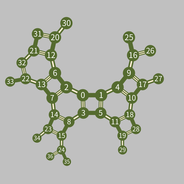
0 is the initial vertex, the number of white strips in an edge indices the type of it (no white strips for \(s_0\), one for \(s_1\) and two for \(s_2\)).
It’s worth noting that one can easily read the shortlex word representation of any vertex \(v\) from the above image, just start from vertex 0, trace a shortest path from 0 to \(v\) (if there are more than one shortest path then always choose the smaller vertex at bifurcaton points) and record the edges along the way. For example there are two paths with shortest length from vetex 0 to vertex 33: \[ \begin{align*}&0\xrightarrow{\ s_1\ }2\xrightarrow{\ s_0\ }6\xrightarrow{\ s_2\ }13\xrightarrow{\ s_1\ }22\xrightarrow{\ s_0\ }33.\\ &0\xrightarrow{\ s_1\ }2\xrightarrow{\ s_2\ }7\xrightarrow{\ s_0\ }13\xrightarrow{\ s_1\ }22\xrightarrow{\ s_0\ }33. \end{align*}\] By concatenating edge labels from left to right we have two words that both map vertex 0 to vertex 33: \(s_1s_0s_2s_1s_0\) and \(s_1s_2s_0s_1s_0\). The first is the shortlex one.
Question 2: How to compute the normal form of the multiplicaiton of two words? How to compute the coset representative of a word for a standard parabolic subgroup?
Again the answer is too long to be included here. A short sketch of the procedure is attached below.
The procedure for computing faces is very similar with the case of edges. The reflections about the \(i\)-th and \(j\)-th mirrors generate a polygon \(f_0\) centered at a vertex of the fundamental triangle. The stabilizing subgroup of \(f_0\) is the standard parabolic subgroup \(\langle i,j\rangle\). Again we find a word representation for each vertex in \(f_0\), apply the words in \(L\) to \(f_0\), and use \(T\) to get the indices of the transformed face.
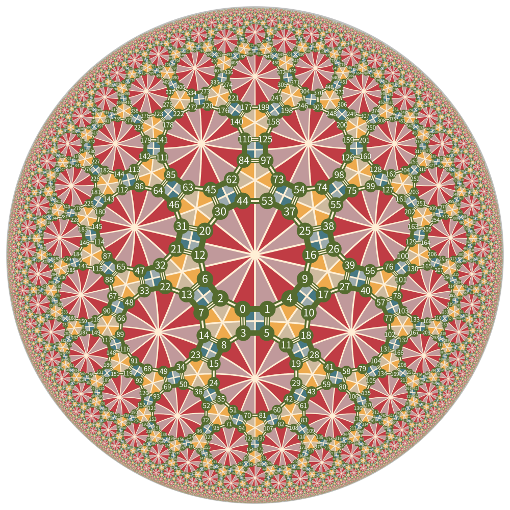
The final image is shown below, it contains 30517 vertices, 42057 edges and 11541 polygons.
About the code
The entire code mainly includes the following functionalities:
- Computation of Coxeter groups. This part is implemented by the
CoxeterGroupclass in thecoxetermodule. The computation of Coxeter groups includes the following aspects:- Compute the minimal root reflection table of the Coxeter group.
- Compute the multiplication of two words in the Coxeter group, and returning the result in its normal form.
- Compute the coset representatives of group elements with respect to a given standard parabolic subgroup, and returning the result in its normal form.
- Compute of the finite state machine that recognizes \(\mathcal{SL}(W)\), minimizing it, and drawing the state machine.
- Tiling drawing. Mainly implemented in the
tiling.pyfile. It includes the following steps:- For a given Coxeter group and specified initial vertex position, calculate the reflection mirrors and fundamental domain.
- Compute the normal forms of all vertices, as well as the connections of edges and faces.
- Apply the words of vertices obtained in the previous step to the initial vertex to obtain the floating-point coordinates of all vertices. These calculations are all performed in one higher dimension, because in the higher dimension all reflections are linear transformations, which avoids the use of affine transformations and inversion. Then project to two dimensions.
- Call the drawing library to draw the tiling.
The drawing of the finite state machine of \(\mathcal{SL}(W)\) requires the use of the
pygraphviz module, which depends on the
graphviz software and libgraphviz-dev.
The minimization of the finite state machine was referenced from Gries’s paper. Gries’s article is excellent, but I think he did not clarify the property of the list that storing the \((B,a)\) pairs.
The drawing of the hyperbolic case uses a third-party library hyperbolic. I’m actually not very satisfied with this library, but I don’t have the energy to write another one at the moment, so I’ll make do for now. The biggest advantage of this library is that it can draw edges with a constant hyperbolic width, namely the so-called hypercycle.
The algorithm for calculating minimal roots is the biggest performance bottleneck in this code. In determining whether a minimal root \(\gamma\) remains a minimal root after a single reflection \(s_\alpha\), the method used is to determine whether \(s_\gamma\) and \(s_\alpha\) generate a finite dihedral group, that is, whether the matrix corresponding to \(s_\gamma s_\alpha\) under the basis \(\Delta\) of simple roots becomes the identity matrix after a certain power. The elements of the matrix are algebraic integers in the cyclotomic field, in the form of \(p(\xi)\), where \(p(x)\) is an irreducible polynomial with integer coefficients, and \(\xi\) is a primitive \(m\)-th root of unity, where \(m\) is twice the least common multiple of all elements in the Coxeter matrix. \(\xi\) can be described by the cyclotomic polynomial \(\Phi_m(x)\). Thus, the computation of the matrix is reduced to polynomial operations in \(\mathbb{Z}[x]/(\Phi_m(x))\). This computational complexity heavily depends on the value of \(m\): for example, for a triangle group like (19, 20, 21), the expression of \(\Phi_m(x)\) is very complicated, and the computation speed is very slow. This is different from the inverse pixel reflection method, whose computational complexity hardly changes with the group.
A more reasonable implementation method can be seen here.
More explainations on the math stuff
In this section I’ll give a short sketch of the core part of the math stuff. This requires you know some basic concepts like geometric realizations of Coxeter groups, Tit’s cone, root systems. These are fairly standard materials and can be found in Humphreys’s book.
Almost everything relies upon a 2d table called reflection table of minimal roots. Again we use group (7, 2, 3) as example:
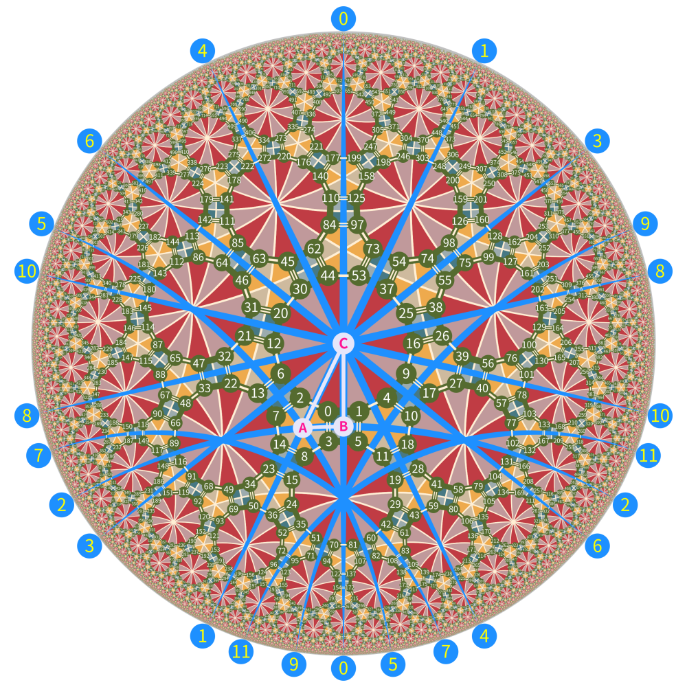
This image is the same with the last one except that it has 12 labelled mirrors, these mirror have particular importance among all roots in the root system: they are the set of minimal roots in the root system.
You can think the root system of \(W\) as all the circular arcs in the diagram, each of which is a reflection mirror. These mirrors are the result of the action of the group \(W\) on the initial mirrors \(AB, AC, BC\) that are the edges of \(\Delta ABC\). Each mirror has two sides, where the side where the fundamental domain \(\Delta ABC\) is located is considered the positive side of the mirror, and the other side is the negative side. The normal vector of the mirror’s positive side gives a positive root, while the normal vector corresponding to the other side is the negative of that positive root (negative root).
We always use a mirror’s positive normal vector (positive root) to represent that mirror.
Intuitively, a minimal root \(\gamma\) is characterized by the following condition: suppose a person stands inside \(\Delta ABC\) looking outward, there exists no mirror \(\beta \neq \gamma\) completely blocking the view of \(\gamma\), preventing the person from seeing any part of \(\gamma\). In other words, this means that if the person wants to walk from the inside of \(\Delta ABC\) to the negatve side of \(\gamma\), and he must cross another mirror \(\beta \neq \gamma\) first, regardless of the path he chooses, then \(\gamma\) is not a minimal root.
Simple roots are necessarily minimal roots, as they are the boundaries of the fundamental domain \(\Delta ABC\), and it is impossible for there to be another mirror blocking between them and the basic region.
The most important fact about minimal root is:
Theorem: The set of minimal roots is finite.
This theorem is the key step in Brink and Howlett’s proof that Coxeter groups are automatic groups.
The reflection table of minimal roots reftable is
defined as follows: it’s a 2d array with its \(i\)-th row correspondes to the \(i\)-th minimal root \(\alpha_i\) and \(j\)-th column correspondes to the \(j\)-th generator \(s_j\). The \((i,j)\)-entry records the action of \(s_j\) on \(\alpha_i\). Let \(\beta=s_j(\alpha_i)\):
- If \(\beta=\alpha_k\) is the \(k\)-th minimal root then set this entry to \(k\).
- If \(\beta\) is a negative root then set this entry to \(-1\).
- Else \(\beta\) is a positive root
but not minimal, set this entry to
None.
The reftable of the (7, 2, 3) group is listed below:
| root | \(s_0\) | \(s_1\) | \(s_2\) |
|---|---|---|---|
| 0 | -1 | 3 | 0 |
| 1 | 4 | -1 | 5 |
| 2 | 2 | 5 | -1 |
| 3 | 6 | 0 | 7 |
| 4 | 1 | 8 | 9 |
| 5 | 9 | 2 | 1 |
| 6 | 3 | 10 | 11 |
| 7 | 11 | 7 | 3 |
| 8 | 10 | 4 | None |
| 9 | 5 | None | 4 |
| 10 | 8 | 6 | None |
| 11 | 7 | None | 6 |
Let \(\Sigma\) be the set of minimal roots of \(G\), all states in the automaton are subsets of \(\Sigma\), the transition rule between the subsets is:
\[S\xrightarrow{\ s_i\ } \{s_i\} \cup (s_i(S)\cup\{ s_i(\alpha_j),j<i\})\cap\Sigma.\]
One can use breadth-first search to build this automaton and use Hopcroft’s algorithm to get a minimized version of it.
The image below shows the subsets of minimal roots for each state in the automaton:

The code for computing the multiplication of a generator and a word is given below:
1 | |
Here \(s\) is a generator and \(w\) is a word in the normal form of the inverse shortlex ordering (invshortlex). The function returns the normal form of \(s\cdot w\) also in the invshortlex ordering. The computations in shortlex can be obtained by doing computations in invshortlex first and then reverse the result back.
注: The intermedian step of doing computations in invshortlex ordering is mainly for keeping consistent with Casselman’s paper.
Finding the coset representative of a given word for a standard parabolic subgroup is quite straight-forward: let \(T\) be the set of generators of this standard parabolic subgroup, the pseudocode for the procedure is given below:
1 | |
Where \(l(\cdot)\) is the length function.
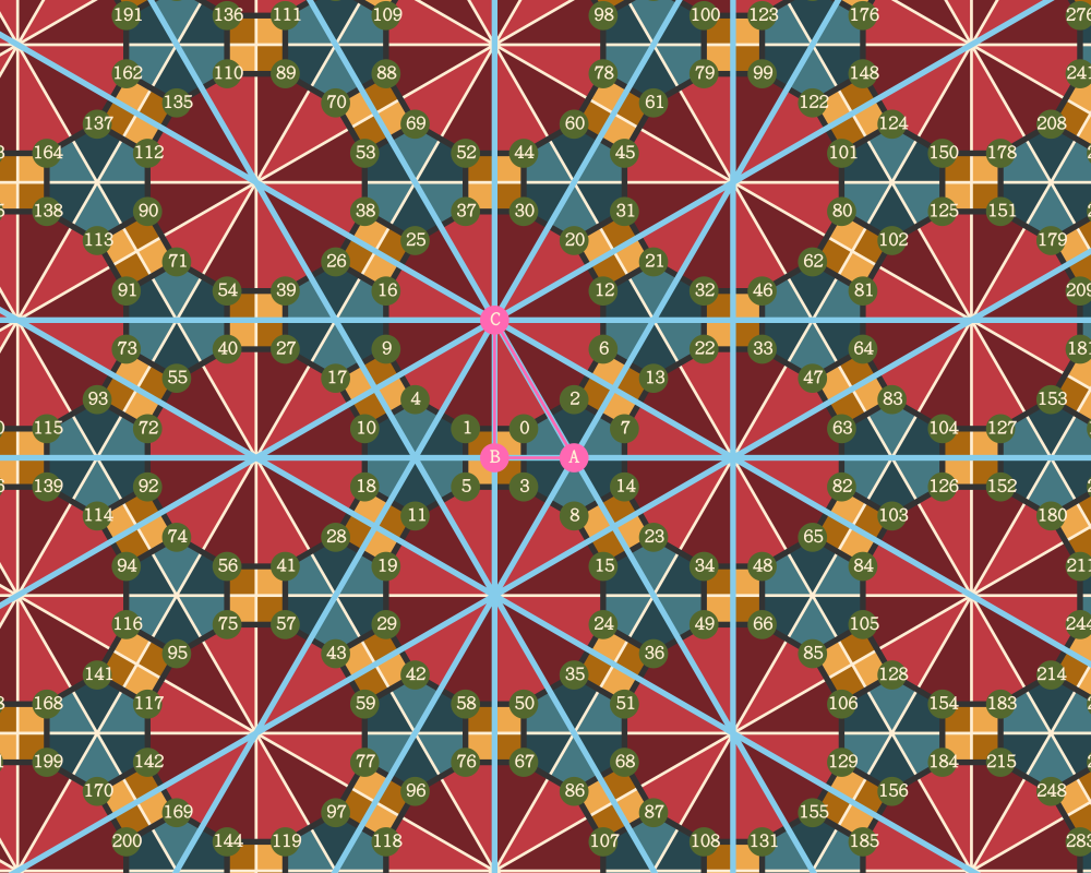
For finite Coxeter groups all positive roots are minimal. For affine Coxeter groups the root system consists of families of parallel affine hyperplanes. In each family there is a pair of minimal roots such that the fundamental domain lies between them and all other mirrors in this family are completely screened off by them hence are not minimal. See the image for (6, 2, 3) (affine \(\widetilde{G}_2\)) for an example:
Automata to perform basic calculations in Coxeter groups, by Bill Casselman.↩︎
Computation in Coxeter groups I. Multiplication, by Bill Casselman.↩︎
Computation in Coxeter groups II. Constructing minimal roots, by Bill Casselman.↩︎
Reflection Groups and Coxeter Groups, by James E. Humphreys.↩︎


