Indra's pearls 中英双语对照
扉页
In the heaven of the great god Indra is said to be a vast and shimmering net, finer than a spider’s web, stretching to the outermost reaches of space. Strung at the each intersection of its diaphanous threads is a reflecting pearl. Since the net is infinite in extent, the pearls are infinite in number. In the glistening surface of each pearl are reflected all the other pearls, even those in the furthest corners of the heavens. In each reflection, again are reflected all the infinitely many other pearls, so that by this process, reflections of reflections continue without end.
在印度教主神因陀罗的梵天之中,悬有一张璀璨绝伦的珍珠宝网,其纤细更胜蛛丝,绵延至宇宙的终极边际。这轻若云烟的罗网间,每一经纬交汇处皆垂缀明珠,因法界无尽,故明珠无量。每颗宝珠的莹润光华中,俱现十方世界一切珠影,纵使远在梵天极隅之珠亦纤毫毕现。更妙者,珠中所映万千珠影,复现重重无尽珠光,如镜镜相照,光光互摄,遂成华严玄境,映现大千世界之无穷法界。
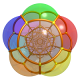
Cover picture: A mathematically generated picture foretold in the Buddhist myth of Indra’s net? We sometimes call these Klein Bubbles. The smallest ones are sehr klein.
封面图片. 这幅由数学生成的瑰丽图案,是否暗合了佛教因陀罗网的古老寓言?我们称之为”克莱因泡泡”,其中最小的泡泡在德语中恰被称作 “sehr klein” (“意为极小”)。
前言
这是什么类型的书?
This is a book about serious mathematics, but one which we hope will be enjoyed by as wide an audience as possible. It is the story of our computer aided explorations of a family of unusually symmetrical shapes, which arise when two spiral motions of a very special kind are allowed to interact. These shapes display intricate ‘fractal’ complexity on every scale from very large to very small. Their visualisation forms part of a century-old dream conceived by the great German geometer Felix Klein. Sometimes the interaction of the two spiral motions is quite regular and harmonious, sometimes it is total disorder and sometimes and this is the most intriguing case - it has layer upon layer of structure teetering on the very brink of chaos.
这是一本关于严谨数学的著作,但我们希望尽可能多的读者都能从中获得乐趣。本书讲述了我们借助计算机,对一类具有非同寻常对称性的图形进行探索的过程。这些图形源自两种特殊螺旋运动的相互作用,展现出在从宏观到微观各个尺度上都极为复杂的“分形”结构。它们的可视化工作实现了德国伟大几何学家菲利克斯·克莱因一个百年前的数学梦想。有时候,这两种螺旋运动的相互作用是规律而和谐的;有时则是完全无序的,最引人入胜的是它们在秩序与混乱的临界状态下,层层结构交织,令人着迷。
As we progressed in our explorations, the pictures that our computer programs produced were so striking that we wanted to tell our tale in a manner which could be appreciated beyond the narrow confines of a small circle of specialists. You can get a foretaste of their variety by taking a look at the Road Map on the final page. Mathematicians often use the word ‘beautiful’ in talking about their proofs and ideas, but in this case our judgment has been confirmed by a number of unbiassed and definitely non-mathematical people. The visual beauty of the pictures is a veneer which covers a core of important and elegant mathematical ideas; it has been our aspiration to convey some of this inner aesthetics as well. There is no religion in our book but we were amazed at how our mathematical constructions echoed the ancient Buddhist metaphor of Indra’s net, spontaneously creating reflections within reflections, worlds without end.
随着我们探索的深入,计算机程序生成的几何图像展现出令人震撼的数学美感,这促使我们渴望以一种超越专业圈子,为更广泛读者所欣赏的方式来讲述这个故事。读者可以通过书末的“探索路线图”先睹为快,感受这些图像的多样风貌。
数学家在谈论他们的证明理念时常常使用“美”这个词,但这一次,不只是我们这样认为——许多并不具数学背景的外行人也认同这些图像具有非凡的美感。图像的视觉美只是一层表面,它所覆盖的内核是重要而优雅的数学思想;我们也希望能够传达这种深层次的美。
虽然本书并不涉及宗教,但我们惊讶地发现,我们的数学结构与佛教“因陀罗网”这一古老隐喻之间产生了意外的共鸣,层层反射自发地衍生出无尽的宇宙。
Most mathematics is accessible, as it were, only by crawling through a long tunnel in which you laboriously build up your vocabulary and skills as you abstract your understanding of the world. The mathematics behind our pictures, though, turned out not to need too much in the way of preliminaries. So long as you can handle high school algebra with confidence, we hope everything we say is understandable. Indeed given time and patience, you should be able to make programs to create new pictures for yourself. And if not, then browsing through the figures alone should give a sense of our journey. Our dream is that this book will reveal to our readers that mathematics is not alien and remote but just a very human exploration of the patterns of the world, one which thrives on play and surprise and beauty.
大多数数学的学习过程就像是在一条漫长的隧道中缓慢前行。在这个过程中,你不断积累词汇和技巧,一步步抽象出对世界的理解。然而,本书图像背后的数学却并不需要太多前置知识。只要你能自信地掌握高中代数,我们相信你能理解书中的所有内容。事实上,若有足够的时间和耐心,你应该能编写程序,自己创造新的图像。即使不这样,仅仅浏览这些图像,也能感受到我们这段旅程的魅力。我们的梦想是通过这本书让读者意识到,数学并非遥远而陌生的事物,而是人类探索世界规律的一种方式,是对世界中各种模式的追寻,它源于游戏、惊喜与美的激发。
我们是如何开始写它的?
David M.’s story. This book has been over twenty years in the writing. The project began when Benoit Mandelbrot visited Harvard in 1979/80, in the midst of his explorations of complex iteration - the ‘fractals’ known as Julia sets - and the now famous ‘Mandelbrot Set’. He had also looked at some nineteenth century figures produced by infinite repetitions of simple reflections in circles, a prototypical example of which had fascinated Felix Klein. David W. and I pooled our expertise and began to develop these ideas further in the Kleinian context. The computer rapidly began producing pictures like the ones you will find throughout the book.
戴维·芒福德(David Mumford)的故事。本书的写作历时二十余年。项目的起点可以追溯到 1979/80 年,当时贝努瓦·曼德布罗特(Benoit B. Mandelbrot)正在访问哈佛大学。彼时他正在探索复迭代系统——即后来被称为朱利亚集的“分形”以及如今广为人知的“曼德布洛特集合”。在此期间,曼德布罗特还研究了一些 19 世纪的图形,这些图形是通过圆反射的无限迭代所生成的,其中一个原型曾经让菲利克斯·克莱因(Felix Klein)深感着迷。大卫·怀特(David W.)和我结合了各自的专业知识,开始在克莱因群的框架下进一步发展这些想法。计算机很快就生成了类似本书中随处可见的那些图像。
What to do with the pictures? Two thoughts surfaced: the first was that they were unpublishable in the standard way. There were no theorems, only very suggestive pictures. They furnished convincing evidence for many conjectures and lures to further exploration, but theorems were the coin of the realm and the conventions of that day dictated that journals only publish theorems. The second thought was equally daunting: here was a piece of real mathematics that we could explain to our non-mathematical friends. This dangerous temptation prevailed, but it turned out to be much, much more difficult than we imagined.
这些图像该如何处理呢?我脑海中浮现出两个念头:首先,它们无法以传统方式发表。它们没有定理,只有一些极具启发性的图像。虽然它们为许多猜想提供了令人信服的证据,也为进一步探索指引了方向,但定理才是数学界通行的“硬通货”,而当时的惯例是,期刊只发表包含定理的文章。
第二个念头同样令人生畏:这是一段真正的数学内容,而我们竟然可以把它讲给非数学背景的朋友听。这种危险的诱惑最终占了上风,但我们很快发现,这远比我们想象的要困难得多。
We persevered off and on for a decade. One thing held us back: whenever we got together, it was so much more fun to produce more figures than to write what Dave W. named in his computer TheBook. I have fond memories of traipsing through sub-zero degree gales to the bunker-like supercomputer in Minneapolis to push our calculations still further. The one loyal believer in the project was our ever-faithful and patient editor, David Tranah. However, things finally took off when Caroline was recruited a bit more than a decade ago. It took a while to learn how to write together, not to mention spanning the gulfs between our three warring operating systems. But our publisher, our families and our friends told us in the end that enough was enough.
我们断断续续坚持了十年。最大的障碍是,每次见面时,大家都觉得创作新图比写 David W. 在他的电脑里命名为 “The Book” 的那本书要有趣得多。我至今仍清晰记得,在明尼阿波利斯刺骨的寒风中,我们跋涉到堡垒般的超级计算机中心,只为将计算推向新的极限。始终对这个项目抱有信心的,是我们忠诚而耐心的编辑 David Tranah。但真正的转折点,是十多年前 Caroline 的加入。我们花了好一阵子才学会如何一起写作,更别提如何在三个“势不两立”的操作系统之间架起桥梁。不过最终,我们的出版商、家人和朋友都对我们说:够了,该收尾了。
You know that ‘word problem’ you hated the most in elementary school? The one about ditch diggers. Ben digs a ditch in 4 hours, Ned in 5 and Ted in 6. How long do they take to dig it together? The textbook will tell you 1 hour, 37 minutes and 17 seconds. Baloney! We have uncovered incontrovertable evidence that the right answer is hours. This is a deep principle involving not merely mathematics but sociology, psychology, and economics. We have a remarkable proof of this but even Cambridge University Press’s generous margin allowance is too small to contain it.
你还记得你小学时最讨厌的那道“应用题”吗?就是关于挖沟工人的那题。Ben 4 小时能挖完一条沟,Ned 需要 5 小时,Ted 要 6 小时。那他们一起挖,要多久才能挖完?课本会告诉你答案是 1 小时 37 分 17 秒。胡说八道!我们已经通过实践得到了确凿的证据,真正的耗时应该是 4 + 5 + 6 = 15 小时。这背后蕴藏着一个深刻的原理,不仅仅涉及数学,还牵扯到社会学、心理学和经济学。我们有一个精彩绝伦的证明过程,但即使是剑桥大学出版社那慷慨的版面,也无法容纳它。
David W.’s story. This is a book of a thousand beginnings and for a long time apparently no end. For me, though, the first beginning was in 1979 when my friend and fellow grad student at Harvard Mike Stillman told me about a problem that his teacher David Mumford had described to him: Take two very simple transformations of the plane and apply all possible combinations of these transformations to a point in the plane. What does the resulting collection of points look like?
Of course, the thing was not just to think about the shapes but to actually draw them with the computer. Mike knew I was interested in discrete groups, and we shared a common interest in programming. Also, thanks to another friend and grad student Max Benson, I was alerted to a very nice C library for drawing on the classic Tektronix 4014 graphics terminal. The only missing ingredient was happily filled by a curious feature of a Harvard education: I had passed my qualifying exams, and then I had nothing else to do except write my doctoral thesis. I have a very distinct memory of feeling like I had a lot of time on my hands. As time has passed, I have been astonished to discover that that was the last time I felt that way.
David W. 的故事。这是一本拥有千百种开端、却似乎长久没有结局的书。对我来说,最初的开端是在 1979 年,那时我在哈佛的朋友、也是研究生同学的 Mike Stillman 跟我讲了一个问题,这是他的老师 David Mumford 描述给他的:取平面上的两种非常简单的变换,将这些变换以各种可能的组合作用在平面上的某个点上。最终得到的这一系列点组成的集合,会是什么样子呢?
当然,事情不仅仅是思考这些图形的形状,而是要真正用计算机把它们画出来。Mike 知道我对离散群感兴趣,我们在编程方面也有共同爱好。此外,多亏了另一位朋友兼研究生 Max Benson 的提醒,我发现了一个非常棒的 C 语言库,可以在经典的 Tektronix 4014 图形终端上进行绘图。最后一个缺失的要素,恰好被哈佛教育中一个颇为特别的安排所填补:我已经通过了资格考试,接下来除了写博士论文之外,几乎没有其他事可做。我清楚地记得当时有一种“手头时间充裕”的感觉。随着时间流逝,我愈发惊讶地意识到,那竟然是我最后一次有那种感觉。
Anyway, as a complete lark, I tagged along with David M. while he built a laboratory of computer programs to visualize Kleinian groups. It was a mathematical joy-ride. As it so happened, in the summer of 1980 , there was a great opportunity to share the results of these computer explorations with the world at the historic Bowdoin College conference in which Thurston presented his revolutionary results in three-dimensional topology and hyperbolic geometry. We arranged for a Tektronix terminal to be set up in Maine, and together with an acoustically coupled modem at the blazing speed of 300 bits per second displayed several limit sets. The reaction to the limit curves wiggling their way across the screen was very positive, and several mathematicians there also undertook the construction of various computer programs to study different aspects of Kleinian groups.
That left us with the task of writing an explanation of our algorithms and computations. However, at that point it was certainly past time for me to complete my thesis. Around 1981, I had the very good fortune of chatting with a new grad student at Harvard by the name of Curt McMullen who had intimate knowledge of the computer systems at the Thomas J. Watson Research Center of IBM, thanks to summer positions there. After roping Curt in, and at the invitation and encouragement of Benoit Mandelbrot, Curt and David M. made a set of extremely high quality and beautiful black-and-white graphics of limit sets. I would like to express my gratitude for Curt’s efforts of that time and his friendship over the years; he has had a deep influence on my own efforts on the project.
总之,出于一种完全随性的心态,我跟着 David M. 一起参与了一个项目,他正在构建一个用于可视化 Kleinian 群的计算机程序实验室。这段经历堪称一次数学上的狂欢之旅。恰巧在 1980 年夏天,出现了一个极好的机会,可以在一场意义非凡的会议上向世人展示这些计算机探索的成果——那就是在鲍登学院(Bowdoin College)举办的历史性会议上,Thurston 发表了他在三维拓扑和双曲几何方面的革命性成果。我们设法在缅因州安装了一台 Tektronix 终端,并通过一台声耦合调制解调器,以惊人的 300 比特每秒的速度,展示了多个极限集。当这些极限曲线在屏幕上蜿蜒浮现时,反响非常热烈。与会的几位数学家也纷纷投身其中,开始构建各类计算机程序,以研究 Kleinian 群的不同方面。
接下来,我们需要撰写一份关于我们算法和计算过程的说明。然而,那时我确实已经到了必须完成论文的最后期限了。大约在 1981 年,我非常幸运地结识了哈佛的一位新晋研究生 Curt McMullen,他因为暑期曾在 IBM 的 Thomas J. Watson 研究中心工作,对那里的计算机系统非常熟悉。在 Benoit Mandelbrot 的邀请与鼓励下,我拉上了 Curt 一起参与项目,Curt 和 David M. 一同制作了一组非常高质量且精美的极限集黑白图像。在此,我要感谢 Curt 当时的辛勤付出,以及多年来给予我的友谊;他对我在这个项目上的努力产生了深远的影响。
Unfortunately, as we moved on to new and separate institutions, with varying computing facilities, it was difficult to maintain the programs and energy to pursue this project. I would like to acknowledge the encouragement I received from many people including my friend Bill Goldman while we were at M.I.T., Peter Tatian and James Russell, who worked with me while they were undergraduates at M.I.T., Al Marden and the staff of the Geometry Center, Charles Matthews, who worked with me at Oklahoma State, and many other mathematicians in the Kleinian groups community. I would also like to thank Jim Cogdell and the Southwestern Bell Foundation for some financial support in the final stages. The serious and final beginning of this book took place when Caroline agreed to contribute her own substantial research work in this area and her expository gifts, and also step into the middle between the first and third authors to at least moderate their tendency to keep programming during our sporadic meetings to find the next cool picture. At last, we actually wrote some text.
遗憾的是,随着我们各自前往新的、彼此独立的机构,计算设施也各不相同,这使得我们难以维持继续推进这个项目所需的程序和热情。我想对许多人表达感谢,他们给予了我鼓励,包括我在麻省理工时的朋友比尔·戈德曼,以及在本科期间与我一同工作的彼得·塔廷和詹姆斯·拉塞尔,还有几何中心的艾尔·马登和工作人员,曾与我在俄克拉荷马州立大学共事的查尔斯·马修斯,以及许多来自克莱因群研究领域的数学家。我还要感谢吉姆·科格德尔和西南贝尔基金会在本书最后阶段给予的一些资金支持。
这本书真正意义上的严肃开端,是在卡罗琳同意贡献她在该领域的重要研究成果和她出色的讲解才能之后。同时,她还在第一作者和第三作者之间起到了“缓冲”作用——至少能抑制他们在我们偶尔聚会时总想继续编程、寻找下一幅炫酷图像的冲动。最终,我们终于开始真正动笔写作了。
We have witnessed a revolution in computing and graphics during the years of this project, and it has been difficult to keep pace. I would also like to thank the community of programmers around the world for creating such wonderful free software such as TEX, Gnu Emacs, X Windows and Linux, without which it would have been impossible to bring this project to its current end.
During the years of this project, the most momentous endings and beginnings of my life have happened, including the loss of my mother Elizabeth, my father William, and my grandmother and family’s matriarch Elizabeth, as well as the birth of my daughters Julie and Alexandra. I offer my part in these pictures and text in the hope of new beginnings for those who share our enjoyment of the human mind’s beautiful capacity to puzzle through things. Programming these ideas is both vexing and immensely fun. Every little twiddle brings something fascinating to think about. But for now I’ll end.
在这个项目进行的这些年里,我们见证了计算和图形领域的一场革命,步伐之快令人难以跟上。我也想感谢全球程序员社区,他们创造了如此出色的免费软件,如 TeX、Gnu Emacs、X Windows 和 Linux。没有这些软件,这个项目根本无法走到今天这一步。
在这个项目进行的岁月里,我人生中最重大的结束与开始也相继发生了:我失去了母亲伊丽莎白、父亲威廉、祖母兼家族的女族长伊丽莎白,也迎来了我两个女儿朱莉和亚历山德拉的出生。我献上这些图画与文字,是希望在新的开始中,与同样热爱人类思维之美的人们分享这份乐趣。将这些思想转化为程序既令人头疼,又妙趣横生。每一个微小的调整,都会带来值得深思的趣味。不过,现在,我将告一段落。
Caroline’s story. I first saw some of David M. and David W.’s pictures in the mid-80s, purloined by my colleague David Epstein on one of his periodic visits to the Geometry Center in Minneapolis. I was struck by how pretty they were - they reminded me of the kind of lace work called tatting, which in another lifetime I would have liked to make myself.
I presumed that everyone else understood all about the pictures, and didn’t pay too much attention, until a little while later Linda Keen and I were looking round for a new project. I had spent many years working on Fuchsian groups (see Chapter 6), and was wanting something which would lead me in to the Kleinian realm where at that time it was all go, developing Thurston’s wonderful new ideas about three-dimensional non-Euclidean geometry (see Chapter 12). By that time, I had somehow got hold of Dave W.’s preprint which described the explorations reported in Chapter 9. I suggested to Linda that it might fit the bill.
卡罗琳的故事。我第一次看到 David M. 和 David W. 的一些图像是在 80 年代中期,那是我同事 David Epstein 去明尼阿波利斯的几何中心定期访问时偷偷带回来的。我被这些图像的美丽深深吸引——它们让我想起一种叫做梭编(tatting)的蕾丝工艺,如果我换一种人生路径,或许也会喜欢亲手做这种东西。
我原以为其他人都已经完全理解这些图像的意义,因此起初也没有太在意。直到后来,我和 Linda Keen 正在寻找一个新的研究课题。当时我已经在 Fuchs 群(见第 6 章)上工作了很多年,想要转向 Kleinian 群的研究领域——那时这个领域正如火如荼地发展,围绕 Thurston 提出的关于三维非欧几何的奇妙新思想(见第 12 章)。那时,我不知怎么搞到了一份 Dave W. 的预印本,里面描述了第 9 章中提到的探索。我于是向 Linda 提议:或许我们可以从这里入手。
The first year was one of frustration, staring at pictures like the ones in Chapter 9 without being able to get any real handle on what was going on. Then one morning one of us woke up with an idea. We tried a few hand calculations and it seemed promising, so we asked Dave W. to draw us a picture of what we called the ‘real trace rays’. What came back was a rudimentary version of the last picture in this book the one we have called ‘The end of the rainbow’. For me it was more like ‘The beginning of the rainbow’, one of the defining moments of my mathematical life. Here we were, having made a total shot in the dark, having no idea what the rays could mean, but knowing they had absolutely no right to be arranged in such a nice way. It was obvious we had stumbled on something important, and from that moment, I was hooked.
For another year we struggled to fit the rays into the one mathematical straight-jacket we could think of, but it just didn’t quite work. One day, I ran into Curt McMullen and mentioned to him what we were playing with. ‘Real trace’, he pondered, ‘That’s the convex hull boundary’.’ And with that clue, we were off. What Curt had told us was that to understand the two dimensional pictures we had to look in threedimensional non-Euclidean space, real Thurston stuff, as you might say. Finally we were able to verify at least most of the two Dave’s conjectures theoretically.
第一年充满了挫败感,我们盯着第 9 章那样的图看了许久,却始终无法真正理解其中的奥秘。直到某天早上,我们中的一个人突然灵光一现。我们做了一些手工计算,结果看起来很有希望,于是就请 Dave W. 帮我们画一张图,描绘我们所说的“真实迹线射线”(real trace rays)。他给我们画回来的,是本书最后一幅图的雏形——我们称之为“彩虹的尽头”。对我而言,那更像是“彩虹的起点”,是我数学生涯中一个具有决定性意义的时刻。那时我们完全是摸着黑前进,根本不知道这些射线意味着什么,但我们清楚它们绝不可能如此巧妙地排列在一起。这太不可思议了,我们知道自己撞上了某个重要的东西。就在那一刻,我被彻底吸引住了。
接下来的一年里,我们努力尝试将这些射线纳入我们所能想到的某种数学框架中,但始终无法完美契合。某天,我碰巧遇到 Curt McMullen,并向他提起我们正在研究的东西。“真实迹线?”他若有所思地说,“那是凸包的边界。”有了这个提示,我们一下子豁然开朗。Curt 告诉我们,若想理解这些二维图像,我们需要在三维的非欧几里得空间中去观察——说得直白点,就是研究真正的 Thurston 理论。从那以后,我们终于能够在理论上验证 Dave 提出的两个猜想中的大部分内容了。
When the 19th century mathematician Mary Somerville received a letter inviting her to make a translation, with commentary, of Laplace’s great book Mécanique Céléste, she was so surprised she almost returned the letter thinking there must have been some mistake. I suppose I wasn’t quite so surprised to get a letter from David M. asking me to help them write about their pictures, but it wasn’t quite an everyday occurrence either. Although I may perhaps write another book, I am unlikely ever again to have the chance to work on one which will be so much trouble and so much fun.
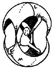
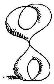
And don’t think this book is the end of the story. If you flick through you will see cartoons of a rather portly character gluing up pieces of rubber into things like doughnuts. In fact all our present tale revolves about ‘one-holed doughnuts with a puncture’. For the last few years, I have been trying to understand what happens when the doughnuts acquire more holes. The main thing I can report is - it’s a lot more complicated! But the same wonderful structures, yet more intricate and inviting, are out there waiting to be tamed.
I would like to thank the EPSRC for the generous support of a Senior Research Fellowship, which has recently allowed me to devote much time to both the mathematical and literary aspects of this challenging project.
当当 19 世纪的数学家玛丽·萨默维尔收到一封信,邀请她翻译并评论拉普拉斯的巨著《天体力学》时,她惊讶得几乎要退回信件,认为一定是出了什么差错。我想,我收到大卫·M. 写信邀请我帮忙为他们的图片撰文时,虽说没有那么惊讶,但这绝非日常小事。尽管我或许还会写另一本书,但恐怕再也不会有机会参与一本既如此费神又如此有趣的书了。
不过别以为这本书就讲完了全部的故事。如果你随手翻一翻,会看到一位略显圆润的角色,正在把橡胶片粘成类似甜甜圈的东西。事实上,我们整个故事都围绕着“打了一个洞的单孔甜甜圈”展开。过去几年里,我一直在试图理解当甜甜圈获得更多洞时会发生什么。我目前唯一能汇报的是——事情会复杂得多!但同样奇妙的结构,更加错综复杂且引人入胜,依然在那里,等着我们去驾驭。
我衷心感谢英国工程与自然科学研究委员会(EPSRC)的慷慨资助,这使我近期能够投入大量时间,专注于这个充满挑战的项目中的数学与文学两个方面。
读者指南
This is a book which can be read on many levels. Like most mathematics books, it builds up in sequence, but the best way to read it may be skipping around, first skimming through to look at the pictures, then dipping in to the text to get the gist and finally a return to understand some of the details. We have tried to make the first part of each chapter relatively simple, giving the essence of the ideas and postponing the technicalities until later. The more technical parts of the discussion have been relegated to the Notes and can be skipped as desired. Material important for later reference is displayed in Boxes.
The first two chapters, on Euclidean symmetries and complex numbers respectively, contain material which may be partially familiar to many readers. We have aimed to present it in a form suited to our viewpoint, at the same time introducing as clearly as possible and with complementary graphics the mathematical terminology which will be used throughout the book. Chapter 3 introduces the basic double spiral maps, called Möbius symmetries, on which all of our later constructions rest. From then on, we build up ever more complicated ways in which a pair of Möbius maps can interact, generating more and more convoluted and intricate fractals, until in Chapters 10 and 11 we actually reach the frontiers of current research. The entire development is summarised in the Road Map on the final page.
这是一本可以从多个层次阅读的书。像大多数数学书一样,它是按顺序逐步展开的,但最佳的阅读方式可能是跳跃式阅读:先快速浏览一遍,看一下插图,然后跳入文本抓住大意,最后再回头理解一些细节。我们尽力让每一章的前半部分相对简单,传达思想的精髓,技术性的内容则推迟到后面再讲。更为技术性的部分被放在了注释中,可以根据需要跳过。对以后参考很重要的内容会以框框的形式展示。
前两章分别讨论了欧几里得对称性和复数,内容对于许多读者来说可能部分熟悉。我们旨在以符合我们视角的形式呈现这些内容,同时尽可能清晰地引入并配以补充图形,介绍本书中将使用的数学术语。第三章介绍了基本的双螺旋映射,称为莫比乌斯对称性,所有后续构建都基于此。从这一章开始,我们逐步构建出越来越复杂的莫比乌斯映射对相互作用的方式,生成越来越复杂、精巧的分形,直到第十章和第十一章,我们实际上达到了当前研究的前沿。整个发展过程在最后一页的路线图中进行了总结。
Words which have a precise mathematical meaning are in bold face the first time they appear. We have not always spelled out the intricacies of the precise mathematical definition, but we have also tried not to say anything which is mathematically incorrect. We have used a small amount of our own terminology, but in so far as possible have stuck to standard usage. Non-professional readers will therefore have to forgive us such terms as quasifuchsian and modular group, while readers with a mathematical training should be able to follow what we mean.
The book is written as a guide to actually coding the algorithms which we have used to generate the figures. A vast set of further explorations is possible for those readers who invest the time to program. This is prime hacking country! Because we hope for a wide variety of readers with many different platforms at their disposal, we have sketched each step in ‘pseudo-code’, the universal programming pidgin.
具有精确数学含义的数学术语在首次出现时以粗体显示。我们并不总是详细阐述这些数学定义的复杂性,但我们也尽量避免说出任何数学上不正确的内容。我们使用了一些自己的术语,但尽可能遵循标准用法。因此,非专业读者可能需要原谅我们使用诸如准富克斯群(quasifuchsian)和模群(modular group)等术语,而具有数学背景的读者应该能够理解我们的意思。
本书的目的是作为编写实际算法的指南,这些算法用于生成我们所展示的图形。对于那些愿意投入时间编程的读者来说,仍有大量的进一步探索空间。这是编程爱好者的天堂!由于我们希望能吸引各种平台上的读者,我们已经以“伪代码”形式勾画了每个步骤,这是编程的通用语言。
Inevitably we have suppressed a good deal of relevant mathematics and anyone wishing to pursue these ideas seriously will doubtless sooner or later have to resort to more technical works. Actually there are no very accessible books about Kleinian group limit sets’, but there are plenty of texts which discuss the basics of symmetry and complex numbers. Some complex analysis books touch on Möbius maps and there is more in modern books on two-dimensional hyperbolic geometry. In the later part of the book we have cited a rather random collection of recent research papers which have important bearing on our work. These are absolutely not meant to be exhaustive, but should serve to help professional readers find their way round the literature.
Finally our Projects need some comment. They can be ignored: we aren’t going to grade them or supply answers! Rather, we intend them as ‘explorations’ to tempt you if you enjoy the material and want to take it further. Some are fairly straightforward extensions or elucidations of material in the text and some involve open-ended questions for which there is no definite answer. A few are definitely research problems. Others again explain details which are needed for full understanding or verification of the more technical points in our story. We have to leave it to the reader to pick and choose which ones suit their taste and mathematical experience.
不可避免地,我们压缩了许多相关的数学内容,任何希望深入研究这些想法的人无疑迟早都需要参考更专业的著作。实际上,关于克莱因群极限集的可读性强的书籍并不多,但有许多书籍讨论了对称性和复数的基础知识。一些复分析的书籍会涉及莫比乌斯变换,现代的二维双曲几何书籍则有更多的相关内容。在本书后部分,我们列举了一些与我们工作密切相关的近期研究论文。这些引用绝不是详尽无遗的,但应该能够帮助专业读者在文献中找到方向。
最后,我们的项目需要做些说明。它们可以被忽略:我们不会给它们打分或提供答案!相反,我们将其作为“探索”,如果你喜欢这些内容并希望深入了解,它们将激发你的兴趣。有些项目是对书中材料的简单扩展或阐述,有些则是开放性问题,没有确切答案。少数是明确的研究问题。还有一些则是解释书中更技术性内容的细节,帮助理解或验证我们的故事中的关键点。我们只能留给读者自己选择,决定哪些项目适合他们的兴趣和数学经验。
致谢
We thank especially our cartoonist Larry Gonick for his uncanny ability to translate a complicated three-dimensional manipulation into an immediately evident cartoon. For historical background we are indebted to the St. Andrews History of Maths web site, tempered with many erudite details and healthy doses of scholarly scepticism from our friends David Fowler and Paddy Patterson. (All remaining errors, are, of course, our own.) Klein’s own book Entwicklung der Mathematikim 19. Jahrhundert has also been an important source. We have read the Hua-Yen Sutra in the translation The Flower Ornament Scripture by Thomas Cleary, Shambhala Publications, 1993, and quotations are reproduced here with thanks. We should like to thank the Mathematics Departments of Brown, Oklahoma State, Warwick, Harvard and Minnesota for their hospitality. We should like to thank the NSF through its grant to the Geometry Center and EPSRC from their Public Understanding of Science budget for financial support. Finally we should like to thank our publisher David Tranah of Cambridge University Press, without whose constant prodding and encouragement this book would almost certainly never have seen the light of day.
我们特别感谢我们的漫画家 Larry Gonick,他拥有将复杂的三维操作转化为一目了然的漫画的神奇能力。关于历史背景,我们要感谢圣安德鲁斯数学历史网站,并且我们特别感谢我们的朋友 David Fowler 和 Paddy Patterson 提供了许多博学的细节和健康的学术怀疑态度。(当然,所有剩余的错误都是我们自己的。)Klein 的《19世纪数学发展》一书也是一个重要的参考来源。我们阅读了 Thomas Cleary 翻译的《华严经》,由 Shambhala 出版社于1993年出版,引用的内容在此谨表示感谢。我们还要感谢布朗大学、俄克拉荷马州立大学、沃里克大学、哈佛大学和明尼苏达大学的数学系对我们的热情接待。感谢美国国家科学基金会(NSF)通过其对几何中心的资助,以及英国工程与物理学研究委员会(EPSRC)从其公共科学传播预算中提供的资助。最后,我们要感谢剑桥大学出版社的出版人 David Tranah,如果没有他不断的督促和鼓励,这本书几乎不可能问世。
7 The glowing gasket
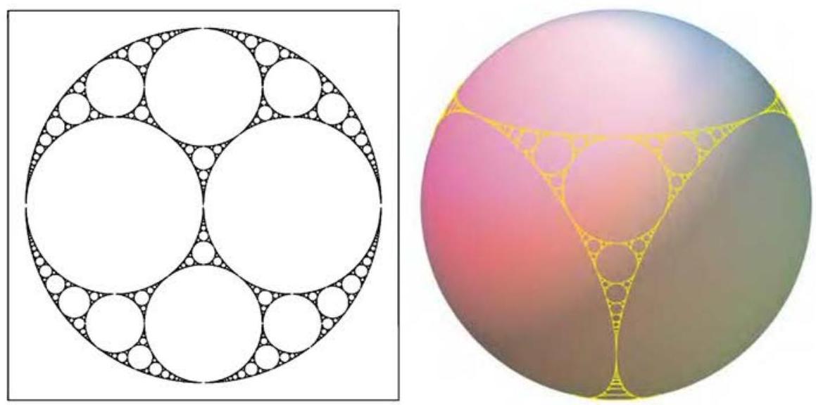
The lacy web in Figure 7.1 is called the Apollonian gasket. Usually, it is constructed by a simple geometric procedure, dating back to those most famous of geometers, the ancient Greeks. We shall start by explaining the traditional construction, but as we shall disclose shortly, the gasket also represents another remarkable way in which the Schottky dust can congeal. The pictures you see here were actually all drawn using a refinement of the DFS algorithm for tangent Schottky circles.
图 7.1 中的镂空结构被称为阿波罗尼奥斯分形。其构造基于一种简单的几何方法,可追溯至古希腊著名的几何学家。我们将首先解释传统的构造方法,但稍后也会揭示,这个分形结构同样展现了肖特基尘埃凝聚的另一种独特形式。此处所见的所有图像,实际上都是通过一种改进版的 DFS 算法绘制的,该算法专门用于处理相切肖特基圆的情况。
The starting point of the traditional construction is a chain of three non-overlapping disks, each tangent to both of the others. A region between three tangent disks is a ‘triangle’ with circular arcs for sides. This shape is often called an ideal triangle: the sides are tangent at each of the three vertices so the angle between them is zero degrees.
The gasket is activated by the fact that in the middle of each ideal triangle there is always a unique ‘inscribed disk’ or incircle, tangent to the three outer circles. It is really better to think of the gasket as a construction on the sphere. Insides and outsides don’t matter any more, so we may as well start with any three mutually tangent circles. You can see lots of disks and incircles in Figure 7.2.
传统构造的起点是三个互不重叠且两两相切的圆盘,呈链状排列。三个相切圆盘围成的区域,形状类似一个以圆弧为边的“三角形”。这种几何图形通常被称为理想三角形:由于其三条边在顶点处相切,因此每个顶点的夹角恰为零度。阿波罗尼奥斯垫片的构造正是由这一特性触发的:每个理想三角形的中心都有且仅有一个内切圆,它同时与这三个外接圆相切。更直观的理解方式是将这一构造置于球面上来考察。这样一来,“内外”之分已无意义,因此我们大可从任意三个两两相切的圆开始。在 图 7.2 中,你会看到许多这样的圆盘及其内切圆结构。
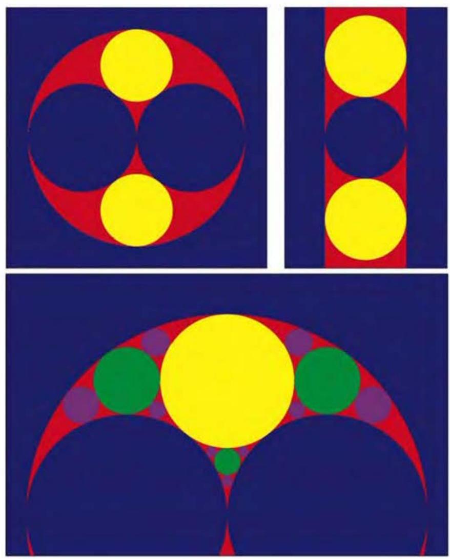
In the figure, we show two initial configurations of three tangent blue disks. When you take out the three blue disks you are left with two red ideal triangles. Each red ideal triangle has a yellow incircle. See how each yellow incircle divides the red triangle into three more triangles.
在图中,我们展示了三个相切的蓝色圆盘的两种初始排布。当你移除这三个蓝色圆盘后,会留下两个红色的理想三角形。每个红色理想三角形各含一个黄色内切圆。仔细观察这些黄色的内切圆如何将红色三角形进一步分割为三个子三角形。
For repetitive people (a necessary quality in this subject, you might say), it is only natural to draw the incircles in these new triangles, resulting, of course, in even more triangles of the same kind. The bottom frame shows this subdivision carried out twice more, with green and then even smaller purple disks. In The Cat in the Hat Comes Back,’ the cat takes off his hat to reveal Little Cat, who then removes his hat and releases Little Cat, who then uncovers Little Cat, and so on. Now imagine there are not one but three new cats inside each cat’s hat. That gives a good impression of the explosive proliferation of these tiny ideal triangles. Carry out this process to infinity, and Voom, the Apollonian Gasket appears.
对于那些乐此不疲的人(或许正是研究这一主题的必备素质),在新三角形中继续绘制内切圆简直是顺理成章的事。这当然会催生出更多相似的三角形。下方的子图展示了这种细分过程再重复两次的结果——先是绿色圆盘,接着是更小的紫色圆盘,密密层层地堆叠起来。这让我想起《戴帽子的猫又来了》中的情节——大猫摘下帽子,露出一只小猫;小猫摘下自己的帽子,又冒出一只更小的小猫;接着更小的小猫再摘帽……如此反复,仿佛无穷无尽。现在,试着想象每顶帽子里不是藏着一只,而是三只小猫,那你就能体会这些微型理想三角形是如何爆炸式增长的了。让这一过程无限延续,砰——阿波罗尼奥斯分形便瞬间跃然眼前。
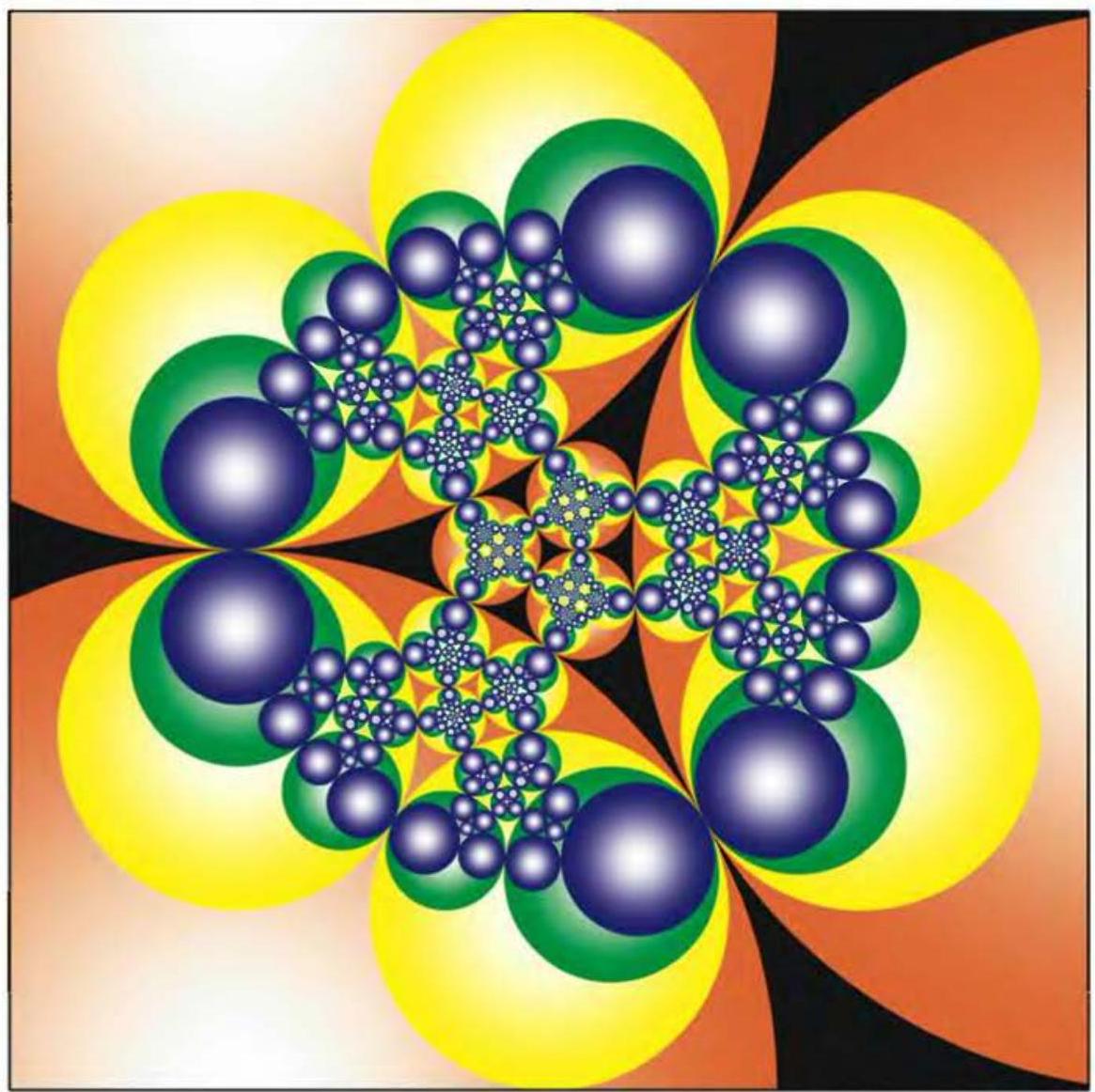
The Apollonian gasket is indeed very pretty, but the reason for introducing it here is that, remarkably, it is also the limit set of a Schottky group made by pairing tangent circles. Exactly the same intricate mathematical object can created by completely different means! You can see better how this works in the beautiful glowing version in Figure 7.3. The solid red circles in this picture are the initial Schottky circles in a very special configuration which we will look at closely in the next section. The glowing yellow limit set can be recognized as the same as the Apollonian gasket of Figure 7.1. The picture was made by pairing four tangent circles arranged in the configuration shown in Figure 7.4. The four circles are tangent not only in a chain; there are also extra tangencies between \(C_a\) and \(C_A\), and between \(C_b\) and \(C_B\).
阿波罗尼奥斯分形确实非常美丽,但我们在此介绍它的原因是:令人惊讶的是,它也是由切圆配对生成的肖特基群的极限集。这一精妙的数学对象,竟然能通过完全不同的方式构造出来!您可以通过 图 7.3 中的荧光渲染图,看到这一过程是如何运作的。图中的实心红色圆环是以一种特殊配置排列的初始肖特基圆(具体分析请参见下一节),其荧黄色的极限集与 图 7.1 中的阿波罗尼奥斯垫片完全一致。这幅图像是通过配对四个相切圆生成的,排列方式如 图 7.4 所示:这些圆不仅形成了链式相切的关系,而且在 \(C_a\) 和 \(C_A\)、\(C_b\) 和 \(C_B\) 之间还存在额外的切点。
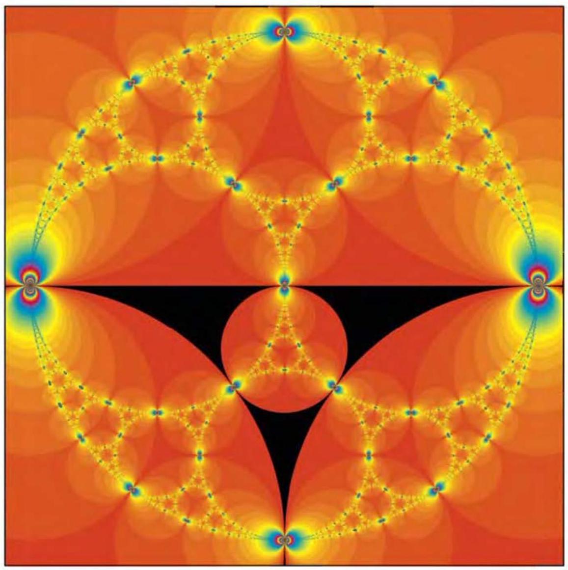
As you iterate the pairing transformations \(a\) and \(b\), the extra tangency proliferates, with the effect that inside each disk \(D\) you see three further Schottky disks tangent to \(D\) and each of the other two. In our version, the circles have been coloured depending on their level, starting with red at the first or lowest level, gradually changing to yellow, green and then blue. The small yellow and blue circles pile up, highlighting the limit set with a mysterious glow.
当你不断迭代配对变换 \(a\) 和 \(b\) 时,额外的切点会迅速增殖。几何上,这表现为:在每个圆盘 \(D\) 内部,都会涌现出三个新的肖特基子圆盘——它们不仅与 \(D\) 相切,而且两两之间也彼此相切。在我们的可视化方案中,圆盘根据迭代的层级依次着色——最底层从红色起步,逐步过渡到黄色、绿色、蓝色。随着黄色和蓝色的小圆盘层层堆叠,极限集被一圈神秘的光晕所笼罩,愈发清晰而引人入胜。
In this chapter, we shall be exploring various features of the gasket. Notwithstanding the extra tangency, it turns out that each limit point is still associated to exactly one or two infinite words in the generators \(a,b,A\) and \(B\). You will be able to make your own version of the glowing gasket by running our DFS algorithm for the group generated by the transformations \(a\) and \(b\). The algorithm draws this complicated lacework as a continuous curve, which is hard to imagine until you see it in progress on a computer screen. The curve snakes its way through the gasket, apparently leaving one region for quite a while until finally weaving its way back. Animation is the true reward of successfully implementing the program we have been learning to build.
在本章中,我们将深入探索垫片结构的各种特性。尽管存在额外的相切关系,但事实证明,每个极限点仍然对应于生成元 \(a, b, A, B\) 所构成的一至两个无限字。通过运行我们为变换群 \(\langle a,b\rangle\) 特别设计的深度优先搜索(DFS)算法,你将能够制作出自己专属的发光垫片。该算法将这种复杂的镂空结构绘制成一条连续的曲线——这种奇妙的生成过程,唯有在计算机屏幕上亲眼目睹,方能真正感受到其变幻莫测之美。曲线如同灵蛇般在 gasket 中蜿蜒穿梭,仿佛要彻底离开某个区域,却又在某个时刻悄然折返。成功实现我们精心构建的程序后,最令人欣喜的收获正是这些跃然屏上的动态演绎。
Apollonius, circa 250-200 BC.
Apollonius, known to his contemporaries as the Great Geometer, lived in Perga, now part of Turkey. One of the giants of Greek mathematics, he was famed for his 8 volume treatise Conics which studied ellipses, hyperbolas and parabolas as sections of a cone by a plane at various angles. His writings swiftly became standard texts in the ancient world. Many are now lost and we know them only through mention in other commentaries, among them works on regular solids, irrational numbers, and approximations to \(\pi\). Ptolemy credits Apollonius with the theory of epicycles on which he based his theory of planetary motion.
One of Apollonius’ lost works is a book called Tangencies, reported to provide methods of constructing circles tangent to various other combinations of lines and circles, for example finding a circle tangent to two given lines and another circle. You can think of the problem of finding the incircle of an ideal triangle in this way. The most difficult problem, that of constructing the two circles tangent to three other given disjoint circles, was probably not solved in ancient times, however Sir Isaac Newton wrote down a proof. According to Pappus, Tangencies gave a formula for the radius of the incircle to an ideal triangle in terms of the radii of the circles which bound its three sides. Be that as it may, exactly such a formula was described by Descartes in 1643, and a version was known in eighteenth century Japan. In fact this formula seems to have been rediscovered many times, most recently by Sir Frederick Soddy, in whose honour the incircles are sometimes known as Soddy circles. Awarded the Nobel prize in 1921, for the discovery of isotopes, Soddy had a natural interest in how to pack spherical atoms of differing size.
Soddy was so taken with the formula that he published it in the unusual form of a poem, which appeared in the journal Nature in 1936. The central part is contained in the middle verse quoted at the head of this chapter. For those who feel more comfortable with symbols, suppose the radii of the chain of three circles are \(a,b\) and \(c\), and that the incircle has radius \(d\). Soddy’s formula is: \[\left(\frac{1}{a}+\frac{1}{b}+\frac{1}{c}+\frac{1}{d}\right)^2=2\left(\frac{1}{a^2}+\frac{1}{b^2}+\frac{1}{c^2}+\frac{1}{d^2}\right).\]
阿波罗尼奥斯,被同时代人誉为伟大的几何学家,生活在佩尔加,即现今土耳其的一部分。作为希腊数学的巨擘之一,他因八卷本专著《圆锥曲线论》而闻名,该著作研究了椭圆、双曲线和抛物线作为平面以不同角度切割圆锥所得截面的性质。其著作迅速成为古代世界的标准教材。许多作品现已遗失,我们仅通过其他评论中的提及了解它们,其中包括关于正多面体、无理数及对 \(\pi\) 的近似值的研究。托勒密将本轮理论归功于阿波罗尼奥斯,这一理论成为他行星运动学说的基础。
阿波罗尼奥斯遗失的著作之一名为《切触》,据记载,该书提供了构建与各种直线和圆组合相切的圆的方法,例如寻找与两条给定直线及另一个圆相切的圆。你可以将寻找理想三角形内切圆的问题视为此类问题。最难的难题,即构建与三个给定且互不相交的圆相切的两个圆,在古代可能并未解决,然而艾萨克·牛顿爵士记录了一个证明。根据帕普斯的说法,《切触》给出了一个公式,用于计算理想三角形内切圆的半径,该半径与限定其三条边的圆的半径有关。尽管如此,笛卡尔在 1643 年确实描述了这样一个公式,且在 18 世纪的日本也已知晓其版本。实际上,这个公式似乎被多次重新发现,最近一次是由弗雷德里克·索迪爵士完成的。为了纪念他,内切圆有时被称为索迪圆。索迪因发现同位素而于 1921 年获得诺贝尔奖,他对如何排列不同大小的球形原子自然产生了兴趣。
索迪对这个公式深深着迷,以至于他以一首诗的形式将其发表,这首诗出现在 1936 年的《自然》杂志上。其核心部分包含在本章开头引用的中间诗句中。对于那些更偏好使用符号的读者,假设三个连锁圆的半径分别为 \(a, b\) 和 \(c\),内切圆的半径为 \(d\)。索迪的公式为:
\[\left(\frac{1}{a}+\frac{1}{b}+\frac{1}{c}+\frac{1}{d}\right)^2=2\left(\frac{1}{a^2}+\frac{1}{b^2}+\frac{1}{c^2}+\frac{1}{d^2}\right).\]
Generating the gasket 生成垫片
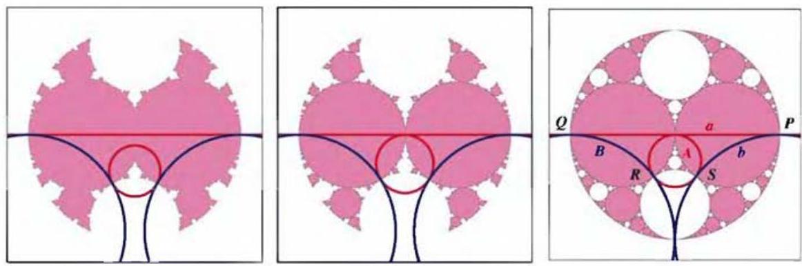
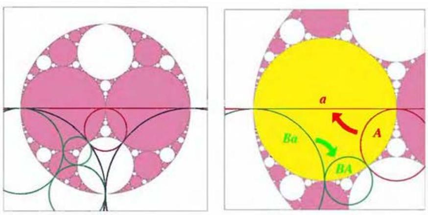
The configuration of tangent circles which produced the gasket is shown in the right frame of Figure 7.4. The picture has been arranged so that \(C_a\) goes through \(\infty\), hence it appears in the figure as a straight line. In addition, \(C_A\) and \(C_a\) are tangent at 0 and \(C_B\) and \(C_b\) are tangent at \(-i\). You can see how this picture is made by creating extra tangencies among a kissing chain of four circles by comparing with the nearby arrangement of four circles in the left hand frame.
生成垫片的相切圆配置如 图 7.4 右图所示。图中特意令圆 \(C_a\) 经过 \(\infty\),从而它在图中呈现为一条直线。此外,我们令圆 \(C_A\) 与 \(C_a\) 在原点 0 处相切,圆 \(C_B\) 与 \(C_b\) 在\(-i\) 处相切。通过与左边图中四个圆的排列进行对比,可以清晰观察到右图通过在四圆相切链中引入额外切点形成的特殊结构。
The generating matrices for the gasket are quite simple: \[a=\begin{pmatrix}1&0\\-2i&1\end{pmatrix}\quad\text{and}\quad b=\begin{pmatrix}1-i&1\\1&1+i\end{pmatrix}.\]
We shall have more to say about how we arrived at these particular formulas later on. Note that \(\mathop{\mathrm{Tr}}{a}=\mathop{\mathrm{Tr}}{b}=2\), so \(a\) and \(b\) are parabolic. Looking at the arrangement of Schottky circles in Figure 7.4, you see the fixed point of \(a\) is 0, the tangency point of the circles \(C_a\) and \(C_A\). In Figure 7.3, you can see two chains of tangent circles nesting down on 0 from above and below. The same phenomenon occurs at \(-i\), the tangency point of \(C_B\) and \(C_b\) and the fixed point of \(b\). Notwithstanding extra tangencies, the generators \(a\) and \(b\) still pair opposite circles in the initial tangent chain \(C_a,C_b,C_A\) and \(C_B\). This means that for nesting circles we still need the commutator condition \(\mathop{\mathrm{Tr}}{abAB}=2\), which is not hard to check.
生成该垫片的矩阵非常简单:
\[a=\begin{pmatrix}1&0\\-2i&1\end{pmatrix}\quad\text{and}\quad b=\begin{pmatrix}1-i&1\\1&1+i\end{pmatrix}.\]
关于这两个特定的矩阵,我们稍后会详细解释它们的推导过程。值得注意的是,由于 \(\mathop{\mathrm{Tr}}{a}=\mathop{\mathrm{Tr}}{b}=2\),因此 \(a\) 和 \(b\) 都是抛物型变换。观察 图 7.4 中 Schottky 圆的排列,可以发现 \(a\) 的不动点是原点 0,即圆 \(C_a\) 和 \(C_A\) 的切点。在 图 7.3 中,你可以看到两条相切的圆链从上下两侧分别向 0 点逐渐嵌套收缩。相同的现象也出现在 \(-i\) 处,这既是圆 \(C_b\) 和 \(C_B\) 的切点,也是变换 \(b\) 的不动点。尽管存在额外的切点,生成元 \(a\) 和 \(b\) 依然将初始的相切链 \(C_a,C_b,C_A,C_B\) 中的圆配对。这意味着要实现圆链的无穷嵌套,我们仍需满足交换子条件 \(\mathop{\mathrm{Tr}}{abAB}=2\),而这一迹值条件并不难验证。
We have been speaking as if there is only one Apollonian gasket, but could we not get different gaskets by starting with different tangent chains? Not really, because it turns out that any chain of three tangent circles can be conjugated to any other three. As you can work out in Project 7.1, this stems from the fact that there is always a Möbius map carrying any three points to any other three. Since the gasket is activated by its initial ideal triangle, and since the procedure at each step consists in adding incircles, a Möbius map which conjugates one ideal triangle to another carries the whole gasket along in its wake.
This explains why it makes sense to talk about the Apollonian gasket, because up to conjugation by Möbius maps there is really only one.
我们此前的讨论似乎一直都默认了阿波罗尼奥斯垫片是独一无二的,但如果我们从不同的初始相切圆链出发,难道不会得到不同的垫片吗?答案是否定的。事实上,任何由三个相切圆组成的链,都可以通过某个莫比乌斯变换转化为另一组(事先给定的)相切圆链。如 项目 7.1 中的推导所示,这一结论的根本原因在于:在复平面上,任意三个不同点总能通过某个莫比乌斯变换映射到任意其它三点。由于垫片的构造源于其初始理想三角形,而每一步的操作都是添加内切圆,因此将一个理想三角形共轭到另一个理想三角形的莫比乌斯变换,会将整个垫片一同带动并映射过去。
这就解释了为什么谈论“阿波罗尼奥斯垫片”是有意义的,因为在莫比乌斯变换的共轭意义下,归根结底,阿波罗尼奥斯垫片只有一个。
另一个著名的垫片版本可以在 图 7.5 中看到。为了得到这个,我们进行了共轭,使得 \(C_a\) 和 \(C_A\) 在 0 处相切,因此它们是垂直线。映射 \(a\) 和 \(b\) 现在在 \(0\) 处有一个固定点。该群的生成元为:
\[a=\begin{pmatrix}2&-i\\-i&0\end{pmatrix}\quad\text{and}\quad b=\begin{pmatrix}1&2\\0&1\end{pmatrix}.\]
Pinching tiles
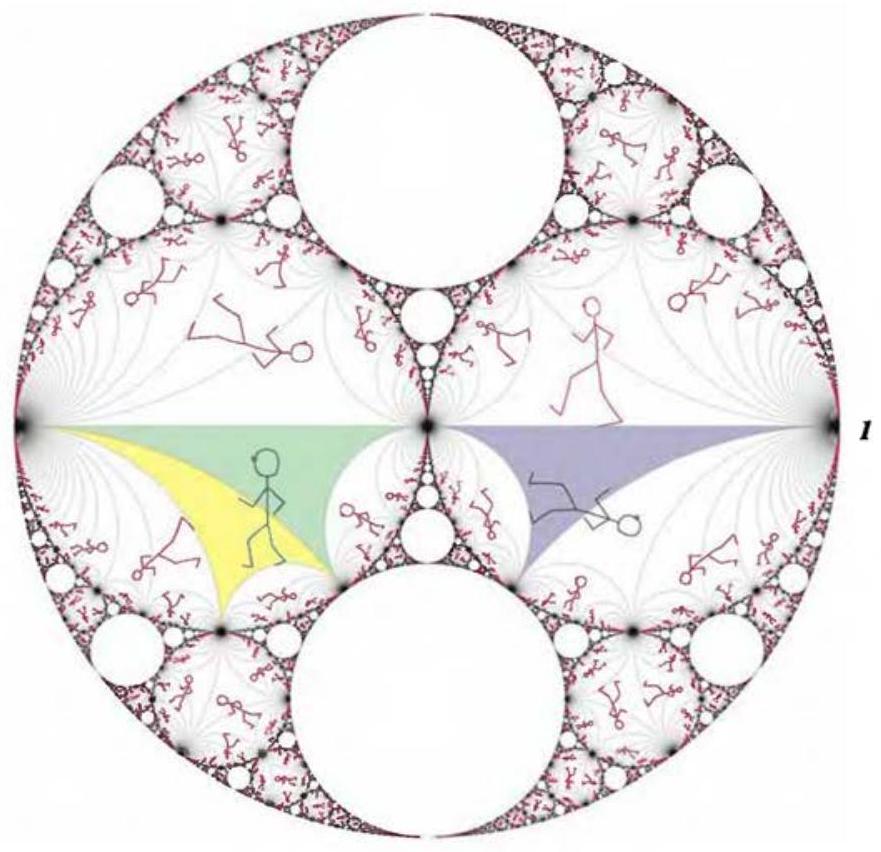
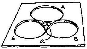
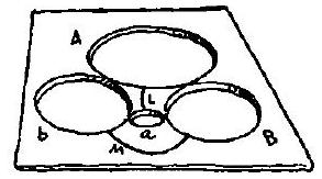
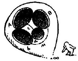
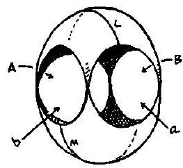
Figure 7.6 is a wonderful picture of what happened when we introduced Dr. Stickler to Apollonius! It is a pretty intricate arrangement, so let’s take a bit of time understanding what has happened to the tiles. To get a grasp on the situation, look back at the three pictures in Figure 7.4, and watch the progression across the three frames. On the left the limit set is a loop or quasicircle, so the ordinary set - what is left when you take away the limit set - has two parts, a pink inside and a white outside. In the central picture, the pink part has collapsed into a myriad of tangent disks, and the red Schottky circles \(C_a\) and \(C_A\) touch at 0. On the right, the gasket group, the ‘horns’ of the pink region have also come together, causing the white outside to fracture into disks as well. Notice how the memory of which was inside and which was outside still persists, because what were the ‘inside’ disks are pink while the ‘outside’ ones are white.
图 7.6 是一幅精彩的画面,生动展现了当我们邀请 Stickler 博士探索阿波罗尼奥斯分形时所发生的奇妙事情!图中的结构相当复杂,因此我们不妨花些时间,仔细剖析图案的变化。要理解这一过程,不妨回顾 图 7.4 的三幅子图,并观察这三帧之间的演变:左图中的极限集是一个回路或拟圆,因此普通集(即去掉极限集后剩下的部分)分为粉色的内部和白色的外部。中间的图中,粉色区域已收缩成无数相切的圆盘,而红色的肖特基圆 \(C_a\) 和 \(C_A\) 在 0 处相切。右图则展示了垫片群,其中粉色区域的“触角”也汇聚在一起,使得白色外部区域也裂解成圆盘。令人惊奇的是,尽管整体结构支离破碎,内外区域仍清晰保留着原始的记忆——曾经“内部”的圆盘依旧是粉色,而“外部”的圆盘依旧是白色。
In each picture, the initial Schottky circles are blue and red. Watch them to follow the fate of the tiles. On the left, as usual for a kissing Schottky group, they surround the central inner four sided tile. If we transported this tile around by the group, we would see a tessellation of the pink region similar to the one in Figure 6.6. (There is also an outer tile, the region outside the four Schottky circles, which as usual you can see more clearly by imagining it on the Riemann sphere.) The inner and outer parts of the ordinary set are invariant under the group, so if you apply any transformation of the group to any tile in the pink region ‘inside’ the limit set, you get another tile which is also ‘inside’.
在每幅图中,最初的 Schottky 圆分别是蓝色和红色。仔细观察它们的变化,有助于追踪瓷砖的去向。在左图中,和典型的“亲吻” Schottky 群一样,这些圆环绕着中央的四边形瓷砖。如果我们将这块瓷砖沿着群的变换移动开来,就会在粉色区域中形成类似于 图 6.6 的镶嵌图案(此外,还有一个外部瓷砖,即位于四个 Schottky 圆之外的区域,通常,通过在黎曼球面上想象它的位置,可以更清楚地看到它的轮廓)。普通集的内部和外部在群作用下各自保持不变,因此,如果对极限集“内部”粉色区域中的某块瓷砖施加群中的某个变换,得到的仍会是另一块位于“内部”的瓷砖。
In the central picture, where \(a\) has become parabolic, the inner tile has been pinched into two halves. Each half-tile is an ideal triangle, with two red sides and one blue. You should think of this pair of triangles as one composite two-part tile. Moved around by the group, the composite tile will cover all the pink circles. There is an outer tile in this picture too, which (on the Riemann sphere) remains in one piece.
On the right, in the gasket group, both \(a\) and \(b\) have been pinched so that now \(C_b\) and \(C_B\) also tuch at \(-i\). Now there are four basic half-tiles. The two pink ones will produce a tiling of the pink circles and the white ones will make a tiling of the white circles. In the glowing gasket picture, these four tiles are black. The upper two ‘horizontal’ ideal triangles are the remnants of the inner Schottky tile, while the lower ‘vertical’ triangle is a remnant of the outer one. If you look carefully, you can just see its twin peeping out in the bottom centre of the page.
在中央的图片中,\(a\) 已变成了抛物型,内部的瓷砖被挤压成了两半。每个半瓷砖都是一个理想三角形,带有两条红边和一条蓝边。你可以把这对三角形视作一个由两部分组成的复合瓷砖。通过群的作用,这个复合瓷砖将覆盖所有的粉色圆盘。图中还有一个外部瓷砖,它在黎曼球面上依然保持完整。
在右侧的垫片图中,\(a\) 和 \(b\) 都被挤压变形,使得 \(C_b\) 和 \(C_B\) 现在也在 \(-i\) 处相切。此时出现了四个基本的半瓷砖。两块粉色的会铺满粉色圆盘,而两块白色的则会铺满白色圆盘。在那幅发光的垫片图中,这四块瓷砖都呈现为黑色。上方的两个“水平”理想三角形是内部 Schottky 瓷砖的残迹,而下方的“垂直”三角形则是外部瓷砖的残迹。仔细观察,你会在页面底部中央隐约发现它的孪生兄弟正悄悄探出头来。
Now we can go back to the picture of Dr. Stickler meeting Apollonius. The party is taking place in the remnants of the ‘pink’ circles. If you compare with the half-tiles in Figure 7.4, something rather odd has happened to Dr. Stickler - when the original tile split in two, his head ended up in the green half-tile and his feet in the blue one. Fortunately, there is a transformation of the group (namely \(B\)) which carries the blue Stickler to the green one, moving the blue half-tile containing the blue feet to the yellow half-tile containing the green feet. Had we not pointed out his difficulties you might not even have noticed that anything was wrong. After gluing the yellow half-tile to the green halftile, the relieved (but still slightly greenish) Dr. Stickler stands reunited in a new and complete tile whose images under the group map to all the Sticklers in the picture.
现在我们可以回到 Stickler 博士与阿波罗尼奥斯相遇的画面。聚会正在“粉色”圆圈的残迹中举行。对照 图 7.4 中的半瓷砖,你会发现 Stickler 博士身上发生了一件相当奇怪的事——当原始瓷砖裂成两半时,原始瓷砖裂成两半时,他的头跑到了绿色半瓷砖里,而他的脚却留在了蓝色半瓷砖上。幸好,群中有一个变换(即 \(B\))可以将蓝色的 Stickler 带到绿色 Stickler 的位置,把装着蓝色脚丫的蓝色半瓷砖挪到装着绿色脚丫的黄色半瓷砖上。要不是我们特意指出这种窘况,你可能根本没发现哪里不对劲。等到黄色半瓷砖和绿色半瓷砖粘合完毕,那位如释重负(却仍然带着一丝“绿意”)的 Stickler 博士终于又完整地站在了一块崭新的瓷砖上。通过群的映射,这块瓷砖的影像铺展开来,构成了画面中所有 Stickler 博士的身影。
And pinching surfaces
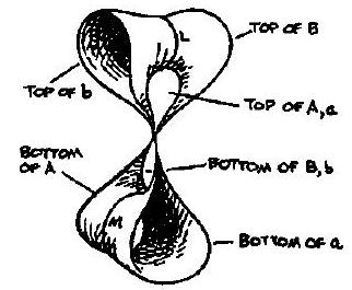
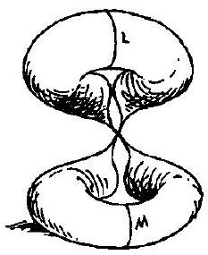
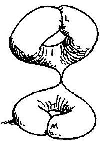
What happened to the tiles in the last section, has, of course, also an interpretation in terms of surfaces. Looking back to the picture on p. 190 which showed how tiles were glued up in a kissing Schottky group, we can work out what happens when we bring the four circles together to make the gasket. It takes a bit of stretching and squeezing to do this, which we have illustrated in Figure 7.7.
The result, shown in the last panel, is our old friend the pretzel with three circles pinched to points or cusps: the waist as in the last chapter and, in addition, loops around the top and bottom tori. Both top and bottom are now ‘spheres’ with three cusps or punctures each. One pair of cusps on each sphere are joined together like ‘horns’, and these two ‘horned spheres’ are themselves joined together at the last two cusps.
上一节中瓷砖的演变过程,当然也可以从曲面角度得到诠释。回顾第 190 页展示的亲吻 Schottky 群的基本域粘合过程的示意图,我们可以推导出当将四个圆粘合为垫片群时会发生什么。这一过程需要一些拉伸和压缩,我们在 图 7.7 中进行了直观展示。
最终结果呈现于最后一幅示意图中,正是我们熟悉的三叶椒盐脆饼造型——三个圆周被压缩为尖点(cusp):其中一个是上一章提到的“腰部”尖点,另外两个则是围绕顶部和底部的环面。此时,顶部与底部都变成了各自有三个尖点(或称穿孔)的”球面”。每个球面上的一对尖点像”犄角”一样连接在一起,而这两个“带角球面”则通过它们剩下的两个尖点相互连接。
The gasket group is called doubly cusped because we have pinched two extra loops, \(a\) and \(b\). It is also sometimes called maximally cusped, because, after all this squeezing, there are no more curves left to pinch. In Chapter 9, we shall see that you can make many variants of the gasket group by imposing more complicated relationships between the curves we choose to pinch on the top and bottom halves of the pinched pretzel.
垫片群被称为双尖群,因为我们挤压了两个额外的环路 \(a\) 和 \(b\)。它也常被称为“极大尖群”,因为经过这般操作后,已不存在可供进一步挤压的曲线。在第九章中我们将看到,通过在挤压后的椒盐卷曲曲面(pretzel)的上下半部之间,对选定挤压曲线施加更复杂的关联约束,可以构造出多种垫片群的变体。
Figure 7.7. Pinching curves. How gluing up the gasket configuration of tangent circles leads to a pair of triply-punctured spheres. The \(a\) and \(b\) curves we have to shrink are are marked \(L\) and \(M\). Instead of pulling the upper and lower partially glued-up cylinders logether right away, as we did in Figure 6.16, it now takes some effort first to twist them relative to each other in such a way that when we glue-up, the dotted loops are in their proper position ready to be shrunk.
图 7.7. 捏合曲线。如何通过粘合垫片的切圆得到一对带有三穿孔球面。需要收缩的 \(a\) 和 \(b\) 曲线分别标记为 \(L\) 和 \(M\)。与 图 6.16 中直接粘合上下圆柱体的操作不同,此时需要先使两者相对扭转,确保粘合时虚线环处于正确位置以便后续收缩。
Tiling the inner disks
Figure 7.6 is made up of lots of disks full of Dr. Sticklers, each tiled by ideal triangles shown in grey. These disks are the remnants of the pink region in Figure 7.4. For most of the rest of this chapter, we shall be occupied with the tiling of just one of these disks. The same tiling fills out the insides of each of the glowing circles in Figure 7.3. The group of symmetries which goes with this very special disk tessellation is called the modular group and has been the well-spring of a huge body of mathematics.
图 7.6 由无数布满 Sticklers 博士身影的圆盘构成,每个圆盘都被灰色的理想三角形所镶嵌。这些圆盘正是 图 7.4 中粉色区域的遗迹。在本章接下来的大部分篇幅里,我们将专注于研究其中一个圆盘的密铺结构。同样的密铺图案也出现在 图 7.3 中每个发光圆圈的内部。这种独特的圆盘镶嵌的对称群称为模群,它一直是众多数学成果的源泉。
Since the tiling in each disk is the same, we may as well focus on the large disk through -1 and 0, shown in yellow in Figure 7.8. To understand how these ideal triangle tiles cover the yellow disk we need to find the subgroup of all the transformations in the gasket group which map the inside of this disk to itself. This subgroup (which is of course also a group in its own right), or any of its conjugates, is what we call the modular group. The basic tile is made up of two ideal triangles, the ones coloured green and yellow in Figure 7.6. The two triangles together form one of our familiar four-sided pinched-off tiles with four circular arc sides. Moved around by the modular group, they tile the whole yellow disk.
由于每个圆盘中的密铺方式相同,我们可以将注意力集中在通过 -1 和 0 的大圆盘上,这在 图 7.8 中以黄色部分表示。为了理解这些理想三角形如何覆盖黄色圆盘,我们需要找出垫片群中所有将圆盘内部映射到自身的变换子群。这个子群(显然,它本身也是一个群),或者它的任何共轭子群,便是我们所称的模群。基本的瓷砖由两个理想三角形组成,即 图 7.6 中绿色和黄色的三角形。这两个三角形合在一起,构成了我们熟悉的四边弧形瓷砖。通过模群的作用,它们密铺了整个黄色圆盘。
We worked out the labels of the boundary circles \(C_a, C_A, C_{BA}\) and \(C_{Ba}\) in Figure 7.8 of the four-sided tile by going to part of the level-two Schottky chain for the gasket group. (You may find it easiest to check the arrangement in a picture like the left frame of Figure 7.4 without all the extra gasket tangencies first.) Notice the four tangency points of these circles are all on the boundary of the yellow disk. As you can see, the four circles form a new chain of tangent circles. As usual, \(a\) pairs \(C_A\) to \(C_a\). In addition, \(BAb\) pairs \(C_{Ba}\) to \(C_{BA}\) because:
\[BAb\left(C_{Ba}\right) = BAb\left(B\left(C_a\right)\right) = BA\left(C_a\right) = B\left(C_A\right) = C_{BA}.\]
Inside the gasket group we have found another mini-chain of four tangent circles, together with a pair of transformations which match them together in pairs!
我们通过研究垫片群的二级 Schottky 链的局部结构,确定了 图 7.8 中四边形瓷砖的边界圆 \(C_a,C_A,C_{BA}\) 和 \(C_{Ba}\) 的标签。(建议首先参考 图 7.4 左图中圆的排列,暂时忽略所有额外的垫片切点,会更容易理解)。值得注意的是,这些圆的四个切点全部位于黄色圆盘的边界上。正如你所见,这四个圆形成了一个新的切圆链。按照惯例,变换 \(a\) 将圆 \(C_A\) 和 \(C_a\) 配对。此外,变换 \(BAb\) 将圆 \(C_{Ba}\) 和 \(C_{BA}\) 配对,原因如下: \[BAb\left(C_{Ba}\right) = BAb\left(B\left(C_a\right)\right) = BA\left(C_a\right) = B\left(C_A\right) = C_{BA}.\] 在垫片群中,我们发现了一个由四个相切圆组成的迷你链,以及一对将它们成对匹配的变换!
This construction shows that the modular group is a new kind of ‘necklace group’, made by disregarding all the rest of the gasket and looking only at the disks produced by acting with \(a\) and \(BAb\) on the four circles which bound the new tile. The new group is generated by the transformations \(a\) and \(BAb\). Indeed in Figure 7.3, you can actually pick out chains of image disks nicely shrinking down onto the glowing limit circle through -1 and 0 . The only difference from the kissing Schottky groups we met in the last chapter is that the two generators pair not opposite circles but adjacent ones. As we shall explain in more detail on p. 213 ff., the image circles shrink because \(a,BAb\) and their product \(aBAb\) are all parabolic.
这一构造表明,模群是一种新型的“项链群”,它是通过忽略垫片的其余部分,仅关注由变换 \(a\) 和 \(BAb\) 作用于新瓷砖边界的四个圆所产生的圆盘而形成的。这个新群由变换 \(a\) 和 \(BAb\) 生成。实际上,在 图 7.3 中,你可以清晰地看到一串映像圆盘,它们逐渐缩小并收敛到经过点 -1 和 0 的发光极限圆上。这与上一章讨论的“接吻式 Schottky 群”的唯一关键时,这两个生成元配对的不是相对的圆,而是相邻的圆。正如我们将在第 213 页及以后章节中详细解释的那样,这些映像圆之所以缩小,是因为 \(a,BAb\) 以及它们的乘积 \(aBAb\) 都是抛物型变换。
The same pattern of pairing circles is repeated all over the gasket. Every pink disk is the image of the yellow one under some element in the gasket group, which conjugates our modular group to another ‘modular group’ acting in the new disk. The white disks are different from the pink ones, because you can never get from pink to white using transformations in the gasket group. However you can still find a chain of four tangent circles matched in the same pattern, as described in Project 7.4.
在垫片的每一个局部区域,都能观察到完全相同的圆配对模式。每个粉色圆盘均可视为黄色圆盘经垫片群中某个变换作用后的像——这个变换元素会将我们原本的模群共轭到一个新的”模群”,而新模群将作用在对应的粉色圆盘上。白色圆盘与粉色圆盘存在本质区别:垫片群中的任意变换都无法将粉色圆盘映射为白色圆盘。不过,我们仍能找到四个相切圆构成的配对链,其模式与前文所述完全一致(具体构造方法详见项目 7.4)。
You might well imagine that we should be set to repeat everything we did in the last chapter. By taking four tangent circles and pairing them in this new pattern we should presumably get a whole new lot of quasifuchsian groups. Not so! It turns out that the rigours imposed by specifying that the two generators and their product are all parabolic actually ‘freeze’ the group. Without any mention of circle chains, we prove in Note 7.1 the remarkable fact that all groups made with pairing conditions like this are, up to conjugation, ‘the same’. What this means in more detail is this. Suppose that \(U\) and \(V\) are any two parabolic Möbius transformations with the property that \(UV\) is also parabolic, and such that the fixed points \({\rm Fix}\,U\) and \({\rm Fix}\,V\) of \(U\) and \(V\) are not the same. Then there is always a conjugating map \(M\) such that: \[ MUM^{-1} = \begin{pmatrix} 1 & 0 \\ -2 & 1 \end{pmatrix}, \quad MVM^{-1} = \begin{pmatrix} 1 & 2 \\ 0 & 1 \end{pmatrix}. \] This explains why there are so many circles in the gasket group, and why you get an identical tiling pattern in each one.
你或许会认为我们需要完全重复上一章的研究过程。通过选取四个相切圆并采用这种新配对模式,我们理应会得到一大堆新的拟富克斯群。然而事实并非如此!事实证明,要求两个生成元及其乘积均为抛物型变换的刚性条件,实质上”冻结”了群的结构。我们在注记 7.1中 不涉及任何圆链概念,证明了如下引人注目的结论:所有满足此类配对条件的群在共轭意义下都是”相同”的。具体而言,设 \(U\) 和 \(V\) 是任意两个抛物型莫比乌斯变换,满足 \(UV\) 仍为抛物型,且两者的不动点 ${},U $与 \({\rm Fix}\,V\)$ 互异,则必存在共轭变换 \(M\) 使得:
\[ MUM^{-1} = \begin{pmatrix} 1 & 0 \\ -2 & 1 \end{pmatrix}, \quad MVM^{-1} = \begin{pmatrix} 1 & 2 \\ 0 & 1 \end{pmatrix}. \] 这解释了垫片群中为什么有如此多的圆圈,以及每个圆内部都会呈现完全相同的密铺图案。
Note
7.1: Uniqueness of the modular group:
注 7.1:模群的唯一性
Suppose that \(U\), \(V\) and \(UV\) are all parabolic (and therefore not the identity!) and the fixed point of \(U\) is \(z_U\) and the fixed point of \(V\) is \(z_V\). We are trying to conjugate \(U\) and \(V\) to the generators of the modular group. We have seen that we can find a Möbius transformation \(M\) that maps \(z_U\) to \(0\) and \(z_V\) to \(\infty\). Conjugating our original transformations \(U\) and \(V\) by \(M\) arranges that \(MUM^{-1}(0) = 0\) and \(MVM^{-1}(\infty) = \infty\), and still the two transformations \(MUM^{-1}\) and \(MVM^{-1}\) are parabolic. Since we can simultaneously conjugate them in this way, we may just as well assume the original transformations \(U\) and \(V\) have fixed points \(0\) and \(\infty\), respectively.
A parabolic transformation that fixes \(\infty\) is always conjugate to any other, up to a minus sign. (See Chapter 3.) Let’s arrange by conjugation and possibly multiplying by -1 that \(V\) corresponds to the matrix \(\begin{pmatrix} 1 & 2 \\ 0 & 1 \end{pmatrix}\). Now all that’s left is \(U\). Since \(U(0)=0\), after again possibly multiplying by -1, we can conclude that the matrix of \(U\) is \[ \begin{pmatrix} 1 & 0 \\ x & 1 \end{pmatrix} \] for some number \(x\).
That brings us to the last hypothesis that \(UV\) is parabolic. Let’s multiply this out:
\[ \begin{pmatrix} 1 & 0 \\ x & 1 \end{pmatrix} \begin{pmatrix} 1 & 2 \\ 0 & 1 \end{pmatrix} = \begin{pmatrix} 1 & 2 \\ x & 1+2x \end{pmatrix}. \]
The trace of \(UV\) under these assumptions is \(2 + 2x\). This is \(\pm 2\) for precisely two values of \(x\), namely, \(x = -2\) and \(x = 0\). In the latter case, \(U\) is the identity, which we are definitely excluding. That means \(x = -2\), and we have shown that \(U\) and \(V\) are simultaneously conjugate to \[ \begin{pmatrix} 1 & 0 \\ -2 & 1 \end{pmatrix} \text{ and } \begin{pmatrix} 1 & 2 \\ 0 & 1 \end{pmatrix}. \] (We may have to multiply one or both matrices by -1 to arrange that they both have trace 2.)
假设 \(U\), \(V\) 和 \(UV\) 均为抛物型变换(因此不是恒等变换!),且 \(U\) 的不动点是 \(z_U\),\(V\) 的不动点是 \(z_V\)。我们的目标是将 \(U\) 和 \(V\) 共轭变换为模群的生成元。我们已经看到,可以找到一个莫比乌斯变换 \(M\),它将 \(z_U\) 映射到 \(0\),\(z_V\) 映射到 \(\infty\)。通过 \(M\) 对原变换 \(U\) 和 \(V\) 进行共轭后,新变换 \(MUM^{-1}\) 将保持 0 不变,\(MVM^{-1}\) 将保持 \(\infty\) 不变,且两者仍为抛物型变换。既然这种共轭可同步完成,我们不妨直接假设原变换 \(U\) 和 \(V\) 的不动点分别是 \(0\) 和 \(\infty\)。
固定 \(\infty\) 的抛物型变换在相差一个符号的意义下彼此共轭(参见第3章)。通过适当共轭及可能的符号调整,可以使 \(V\) 对应于矩阵 \(\begin{pmatrix} 1 & 2 \\ 0 & 1 \end{pmatrix}\)。此时仅需确定 \(U\) 的形式。由于 \(U(0) = 0\),经可能的符号调整后,\(U\) 的矩阵必为: \[ \begin{pmatrix} 1 & 0 \\ x & 1 \end{pmatrix}\quad (x\in\mathbb{C}). \] 接下来验证 \(UV\) 的抛物型条件。计算其乘积:
\[ \begin{pmatrix} 1 & 0 \\ x & 1 \end{pmatrix} \begin{pmatrix} 1 & 2 \\ 0 & 1 \end{pmatrix} = \begin{pmatrix} 1 & 2 \\ x & 1+2x \end{pmatrix}. \] 此时 \(UV\) 的迹是 \(2 + 2x\)。抛物型变换的迹需满足 \(|\mathop{\mathrm{Tr}}|=2\),这恰好对 \(x\) 的两个值成立,即 \(x = -2\) 和 \(x = 0\)。当 \(x=0\) 时,\(U\) 退化为恒等变换(已排除),因此必有 \(x=−2\)。由此可知 \(U\) 和 \(V\) 可共轭于矩阵:
\[ \begin{pmatrix} 1 & 0 \\ -2 & 1 \end{pmatrix} \text{ and } \begin{pmatrix} 1 & 2 \\ 0 & 1 \end{pmatrix} \]
(必要时可对其中一个或两个矩阵取负,以确保其迹均为 2)
The modular group of arithmetic
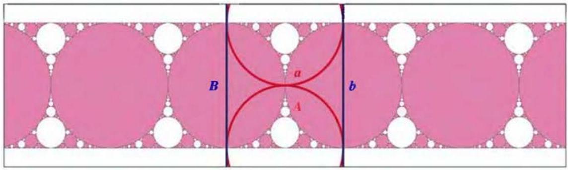
The result just discussed shows that the modular group is conjugate to a very famous group of great importance in number theory. It is made by arranging the four Schottky circles with their tangency points at \(-1,0,1\) and \(\infty\). You can see these, coloured red and green, in the left frame of Figure 7.9. Since one of the tangency points is the point at infinity, two of the circles show up as green vertical lines. These green lines are paired by \(b=\begin{pmatrix}1&2\\0&1\end{pmatrix}\), while the two red circles tangent at 0 are paired by \(a=\begin{pmatrix}1&0\\-2&1\end{pmatrix}\). Notice how \(a\) and \(b\) match adjacent circles in the chain in exactly the pattern of the red and green arrows in Figure 7.8. In fact, as you can easily calculate, \(ab\) is the parabolic transformation \(\begin{pmatrix}1&2\\-2&-3\end{pmatrix}\).
刚刚讨论的结果表明,模群与一个在数论中极为著名且重要的群是共轭的。这个群是通过排列四个肖特基圆生成的,其切点分别位于 \(-1, 0, 1\) 和 \(\infty\)。在 图 7.9 的左图中,这些圆分别以红绿两色呈现。由于其中一个切点是无穷远点,因此有两个圆在图中呈现为绿色的垂直直线。这两条绿色直线由变换 \(b=\begin{pmatrix}1&2\\0&1\end{pmatrix}\) 配对,而在原点 0 处相切的两个红色圆则通过变换 \(a=\begin{pmatrix}1&0\\-2&1\end{pmatrix}\) 配对。请注意,变换 \(a\) 和 \(b\) 对相邻圆的配对方式,恰好与 图 7.8 中红绿箭头所示的模式完全一致。事实上,通过简单的计算即可验证,\(ab\) 是抛物型变换 \(\begin{pmatrix}1&2\\-2&-3\end{pmatrix}\)。
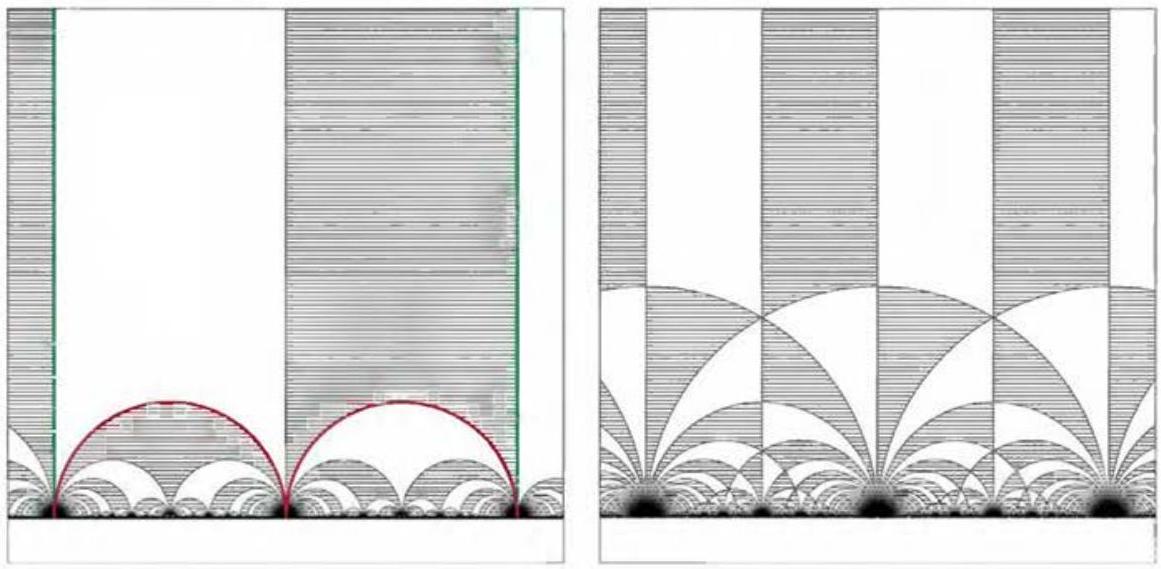
It is no coincidence that the entries of these three matrices are integers. The right frame of Figure 7.9 is a more complicated picture which shows all the symmetries of the tiling on the left. Each ideal triangle has been subdivided into three hatched and three unhatched sub-triangles. (The sub-triangles are not quite ideal, because only one of their angles is 0 .) The group of symmetries of this more complicated tiling is, from the point of view of Möbius maps, the simplest group of all: just the set of all \(2\times 2\) matrices \(\begin{pmatrix}p&q\\r&s\end{pmatrix}\) with integer entries \(p,q,r\) and \(s\) and determinant \(ps-qr\) equal to 1. To distinguish from the group of the left frame, we sometimes call it the full modular group. The matrices in the (smaller) modular group of the left picture are just those matrices with integer entries for which \(q\) and \(r\) are even and \(p\) and \(s\) are odd.
这三个矩阵的元素都是整数,此现象绝非偶然。图 7.9 右侧的复杂图像完整呈现了左侧密铺图案的所有对称性。每个理想三角形都被剖分为三个阴影子三角形和三个非阴影子三角形。(这些子三角形并不完全是理想的,因为它们只有一个角为 0)。从莫比乌斯变换的角度来看,这个更复杂的密铺结构的对称群是最简单的:即所有元素为整数且行列式 \(ps-qr\) 等于 1 的 \(2\times2\) 矩阵 \(\begin{pmatrix}p&q\\r&s\end{pmatrix}\) 构成的集合。为了与左图的对称群区分开来,该群常被称为全模群。而左侧密铺对应的(较小)模群则由满足特殊同余条件的整数矩阵构成——其 \(q\) 与 \(r\) 元素都是偶数,\(p\) 与 \(s\) 元素都是奇数。
There is a very beautiful connection between the modular tessellation and fractions: the points where the ideal triangles meet the real axis are exactly the rational numbers. Although it is something of a digression here, we want to take the time to explain the pattern, which turns out to be indispensible when we come to map making in Chapter 9.
模镶嵌与有理数之间有着极为精妙的联系:理想三角形与实轴交点恰恰是有理数。虽然这一内容在此略显偏离主题,但我们希望花些时间来阐明这个规律,因为它在第 9 章的制图过程中将变得至关重要。
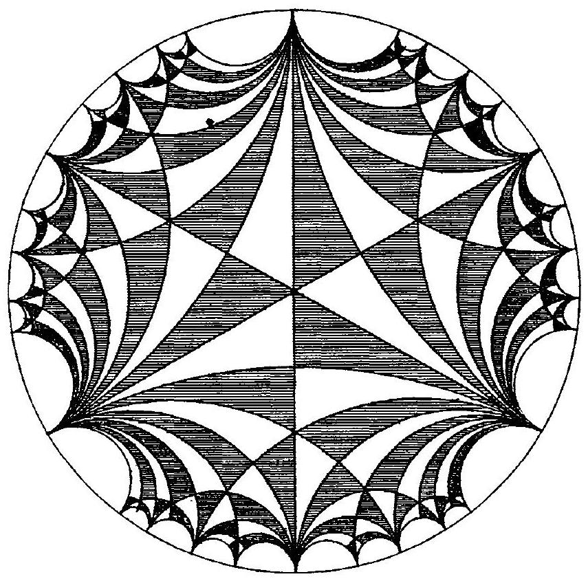
Figure 7.11 shows the first few levels in the modular tessellation. The basic tile is the four-sided region, called an ideal quadrilateral, which was bounded by the coloured lines in Figure 7.9. Images of this ideal quadrilateral are shown bounded by solid arcs. The dotted arcs divide them into the two ideal triangles which we saw, half hatched and half white, on the left in Figure 7.9. As the group acts on the basic tile, we get more and more smaller and smaller tiles nesting down to the real axis. The vertices of all these tiles meet the real axis in points which are all fractions. Several things can be read off from a careful examination of this intricate pattern:
- All vertices of the tiles are rational numbers \(p/q\).
- If \(r/s\) and \(p/q\) are two vertices of the same tile, then \(ps - rq = \pm 1\).
- If \(r/s < p/q\) are the outer two vertices of a tile, then the third vertex between them is \((r + p)/(s + q)\).
Check this out! For instance, between \(2/3\) and \(1/2\), we get \((2 + 1)/(3 + 2)\), that is \(3/5\).
图 7.11 展示了模镶嵌的前几个层级。基本瓷砖是一个四边形,称为理想四边形,它由 图 7.9 中的彩色线条围成。实线弧显示了这个理想四边形的图像,而虚线弧将其分割成两个理想三角形,这两个三角形可以在 图 7.9 的左侧看到,一半是阴影,一半是空白。随着群对基本瓷砖的作用,我们得到越来越多、越来越小的瓷砖,逐层嵌套,直至延伸到实轴。所有这些瓷砖的顶点都与实轴相交,这些交点都是分数。仔细观察这个复杂的图案,我们可以得出以下几个结论:
- 所有瓷砖的顶点都是有理数 \(p/q\)。
- 如果 \(r/s\) 和 \(p/q\) 是同一瓷砖的两个顶点,则 \(ps - rq = \pm 1\)。
- 如果 \(r/s < p/q\) 是同一瓷砖的两个外顶点,那么它们之间的第三个顶点是 \((r + p)/(s + q)\)。
验证一下吧!比如,在 \(2/3\) 和 \(1/2\) 之间,我们得到 \((2 + 1)/(3 + 2)\),即 \(3/5\)。
It’s easy to see why this happens. As we have seen, a typical matrix in the modular group will look like
\[M = \begin{pmatrix} p & q \\ r & s \end{pmatrix}\]
where \(p, q, r\) and \(s\) are integers and \(ps - rq = 1\). If \(M\) acts on the vertices of the initial triangle with vertices \(0 = 0/1, 1 = 1/1\) and \(\infty = 1/0\), then we get the new triangle with vertices \(M(0) = r/s, M(\infty) = p/q\) and \(M(1) = (p + r)/(q + s)\). Assuming all four entries are positive, we have \(r/s < (p + r)/(q + s) < p/q\) (you can see this by multiplying out). This is just what we found in Figure 7.11. If \(p, q, r, s\) are not all positive, there are half a dozen other cases in which the order of the points \(M(0), M(1)\) and \(M(\infty)\) is different but we get the same result. The same thing happens if we start from the other triangle \(M(-1), M(0), M(\infty)\).
这个现象不难理解。我们知道,模群中的一个典型矩阵可以表示为 \[M = \begin{pmatrix} p & q \\ r & s \end{pmatrix},\] 其中 \(p, q, r\) 和 \(s\) 是整数,且满足 \(ps - rq = 1\)。如果矩阵 \(M\) 作用于初始三角形的顶点,该初始三角形的顶点分别是 \(0 = 0/1, 1 = 1/1\) 和 \(\infty = 1/0\),那么变换后的新三角形的顶点将变成 \(M(0) = r/s, M(\infty) = p/q\) 和 \(M(1) = (p + r)/(q + s)\)。假设 \(p,q,r,s\) 都是正数,我们可以验证不等式 \(r/s < (p + r)/(q + s) < p/q\) 成立(通过乘法可轻松验证)。这正是 图 7.11 所示的情况。如果 \(p, q, r, s\) 并非全为正数,还有几种不同的情形,此时点 \(M(0), M(1), M(\infty)\) 的顺序可能会改变,但结果仍然一致。类似地,若从另一个三角形 \(M(-1), M(0), M(\infty)\) 出发,也会得到相同的结论。
Any two fractions \(r/s\) and \(p/q\) such that \(ps - qr = \pm 1\) are called neighbours. Thus any two vertices of an ideal triangle in the modular tessellation are neighbours. If \(p/q\) is a fraction, then, as we explain in Project 7.5, the process of finding its neighbours is essentially Euclid’s two thousand year old algorithm for finding the highest common factor of two numbers, surely one of the most useful and clever algorithms of all time. The rule for finding the ‘next’ point \(\frac{p+r}{q+s}\) between two neighbours is every student’s dream of what addition of fractions should be. This simple form of fraction ‘addition’ is sometimes called Farey addition’, which one might want to symbolise with a funny symbol like:
\[ \frac{p}{q} \oplus \frac{r}{s} = \frac{p + r}{q + s} \]
Farey addition gives a neat way of organising the rational numbers. Instead of the usual way of arranging them in increasing order (which is difficult, because you never know which one should come ‘next’), fractions can be described by a sequence of left or right moves, reflecting the choice at each stage of whether we choose the new pair of neighbours to the right, or the pair of neighbours to the left.
任何两个分数 \(r/s\) 和 \(p/q\),若满足 \(ps - qr = \pm 1\),则称它们为邻居。因此,模群镶嵌中的理想三角形的任意两个顶点都是邻居。如果 \(p/q\) 是一个分数,那么正如我们在项目 7.5 中所解释的那样,寻找其邻居的过程,本质上就是欧几里得两千年前发明的最大公约数算法——这无疑是人类历史上最实用、最巧妙的算法之一。计算两个邻居之间“下一个”点 \(\frac{p+r}{q+s}\) 的规则,正是每个学生心目中理想的分数加法方式。这种简单的分数“加法”有时被称为“法雷加法”(Farey addition),人们或许会用一个有趣的符号来表示它,比如: \[ \frac{p}{q} \oplus \frac{r}{s} = \frac{p + r}{q + s} \]
法雷加法提供了一种巧妙的方式来组织有理数。不像按递增顺序排列那样麻烦(毕竟你很难确定下一个该是谁),分数可以通过一系列左移或右移的操作来描述,这正对应了我们在每一步中选择将新的邻居对放置在左边还是右边的决定。
For positive fractions, the starting point are the two fractions \(0/1\) and \(1/0\), which we can regard as special honourary neighbours because they are connected by a side of our initial triangle, the vertical imaginary axis. Farey addition gives the in-between fraction \(0/1\oplus 1/0=1/1\).
Now we have a choice: go to the ‘left’ and look in the interval between 0 and 1, or go to the ‘right’ and look in the interval between 1 and \(\infty\). Suppose we are aiming for the fraction \(3/5\). Then we turn to the left and apply the Farey addition \(0/1 \oplus 1/1 = 1/2\). At the next stage, we choose the right interval and Farey add to get \(1/2 \oplus 1/1 = 2/3\). Finally, we choose the left interval and Farey add \(1/2 \oplus 2/3 = 3/5\). An exactly similar procedure could be applied to home in on any fraction \(p/q\). Our choice of left-right turns is a driving map: \(3/5\) is given by the instructions ‘left, right, left’. This arrangement of fractions and sequence of right-left moves is closely related to a way of writing fractions as what are called continued fractions, explained in Note 7.2.
对于正分数,我们的起点是两个特殊的分数:\(0/1\) 和 \(1/0\)。我们不妨将它们视作“荣誉邻居”,因为它们由初始三角形的一条边——垂直的虚轴——连接在一起。利用 Farey 加法,我们可以在它们之间找到一个中间分数:\(0/1 \oplus 1/0 = 1/1\)。
接下来,我们需要做出选择:向“左”走,查看 0 到 1 之间的区间;还是向“右”走,查看 1 到 \(\infty\) 之间的区间。假设我们的目标是分数 \(3/5\)。那么我们选择向左,执行 Farey 加法:\(0/1 \oplus 1/1 = 1/2\)。在下一步,我们转向右侧区间,并执行 Farey 加法得到:\(1/2 \oplus 1/1 = 2/3\)。最后,我们再次选择左侧区间,进行 Farey 加法:\(1/2 \oplus 2/3 = 3/5\)。
通过完全相同的步骤,我们可以找到任意分数 \(p/q\)。我们每次选择向左或向右的决策就像一张“导航图”:例如,分数 \(3/5\) 对应的指令是“左、右、左”。这种分数的排列方式和左右转向的序列,与将分数表示为连分数的写法密切相关,详见注释 7.2。
The pairing pattern of the modular group
The modular group is a new kind of ‘necklace group’. It is still made by pairing four tangent circles, and the only difference from the kissing Schottky groups we met in the last chapter is that the generators pair not opposite circles but adjacent ones. Whenever we have an arrangement of paired tangent circles like this, something like the necklace condition on p. 168 must still be true, but because we are pairing the circles in a different pattern, we can expect that different elements must be parabolic to cause the image circles to shrink.
模群是一种新型的“项链群”。它同样由四个相切的圆配对构成,不同之处在于,生成元这次配对的不是相对的圆,而是相邻的圆。每当我们遇到这样的相切圆配对排列时,类似于第 168 页提到的“项链条件”仍然必须成立。不过,由于这次采用了不同的配对模式,我们可以预见,只有某些不同的元素变成抛物型时,映像圆才会缩小。
With the notation of the figure beside Box 20, we have \(a(P) = R\) and \(b(R) = P\), so that the four tangency points of the circles are \(S = \text{Fix}(a)\), \(Q = \text{Fix}(b)\), \(P = \text{Fix}(ba)\), and \(R = \text{Fix}(ab)\). By similar reasoning to that in Chapter 6, in order for the image circles near \(S\) and \(Q\) to shrink, the generators \(a\) and \(b\) must be parabolic. Moreover, \(ba\) must also be parabolic, to make the circles shrink at \(P\). Notice that \(ab\) and \(ba\) are conjugate (since \(b(ab)b^{-1} = ba\)), so saying that \(ab\) or \(ba\) must be parabolic is really one and the same thing. The wonderful thing is, that as we proved in Note 7.1, all groups with these three elements parabolic are automatically conjugate. This is so important to us that we summarize it in Box 20.
Because the pattern of pairing circles is different, so is the arrangement in which the labelled circles are laid down in the plane. The Schottky circles in Figure 7.11 are labelled according to our usual rules, so for example, \(C_{ba}\) still means the image of circle \(C_a\) under the map \(b\). However, if you look carefully, you will see that the order of the circles along the line is not the same as our original order round the boundary of the word tree on p. 104. The labels can be read off in their correct order from the revised version in Figure 7.12. (To see this you will have to twiddle the diagram around so the arrows from the vertex you are interested in are pointing ‘down’ rather than ‘up’.) There is a subtle difference from our original word tree, because there the cyclic order round a vertex was \(a,B,A,b\) while now it is \(a,A,b,B\). The ramifications of this seemingly minor change propagate down the tree.
根据盒 20 旁的图示,我们有 \(a(P) = R\) 且 \(b(R) = P\),因此四个切点分别是:\(S = \text{Fix}(a)\), \(Q = \text{Fix}(b)\), \(P = \text{Fix}(ba)\) 和 \(R = \text{Fix}(ab)\)。类似于第 6 章的推理,为了使靠近 \(S\) 和 \(Q\) 的映像圆缩小,生成元 \(a\) 和 \(b\) 必须是抛物型的。此外,\(ba\) 也必须是抛物型的,才能确保圆在 \(P\) 处缩小。需要注意的是,\(ab\) 和 \(ba\) 是共轭的(因为 \(b(ab)b^{-1} = ba\)),因此说 \(ab\) 或 \(ba\) 必须是抛物型的,实际上是同一回事。奇妙的是,正如我们在注释 7.1 中所证明的,所有包含这三个抛物型元素的群自动共轭。这一点对我们来说非常重要,因此我们在图 20 中专门进行了总结。
由于配对圆的模式不同,标记圆在平面上的排列方式也随之改变。图 7.11 中的 Schottky 圆仍按照我们通常的规则标记,例如,\(C_{ba}\) 依然表示圆 \(C_a\) 在映射 \(b\) 下的像。然而,如果你仔细观察,就会发现这些圆沿着直线的排列顺序与我们最初在边界上的顺序并不相同。
Playing with parameters
I could spin a web if I tried.’ said Wilbur, boasting. ‘Ive just never tried.’
‘Let’s see you do it,’ said Charlotte…
‘OK.’ replied Wilhur. ‘You coach me and I’t’ spin one. It must be a lot of fun to spill a web. How do I start?
“要是我愿意,我也能织网。”威尔伯吹嘘道,“只是我从来没试过。”
“那你来织一个给我们看看吧。”夏洛特说。
“好啊。”威尔伯答道,“你来指导我,我就织一个。织网一定很好玩。我该怎么开始呢?”
As any mathematician who has revealed his (or her) occupation to a neighbour on a plane flight has discovered, most people associate mathematics with something akin to the more agonizing forms of medieval torture. It seems indeed unlikely that mathematics would be done at all, were it not that a few people discover the play that lies at its heart. Most published mathematics appears long after the play is done, cloaked in lengthy technicalities which obscure the original fun. The book in hand is unfortunately scarcely an exception. Never mind; after a fairly detailed introduction to the art of creating tilings and fractal limit sets out of two very carefully chosen Möbius maps, we are finally set to embark on some serious mathematical play. The greatest rewards will be reaped by those who invest the time to set up their own programs and join us charting mathematical territory which is still only partially explored.
正如任何一位曾在飞机上向邻座透露自己职业的数学家都会发现的那样,大多数人对数学的印象,似乎与某种中世纪酷刑的痛苦体验无异。倘若不是有少数人发现了数学的核心妙趣,数学恐怕早已无人问津。大多数已发表的数学成果,往往是在趣味探索结束许久之后才浮出水面的,而那些冗长繁复的技术细节,往往掩盖了最初的乐趣。遗憾的是,手头的这本书也未能完全例外。不过,别担心——在颇为详尽地介绍了如何用两个精心挑选的莫比乌斯变换来构造密铺图案和分形极限集之后,我们终于可以开始一场真正的数学探险了。那些愿意投入时间亲手编写程序、与我们一道探索这片尚未完全揭示的数学版图的读者,定将收获最丰厚的回报。
All the limit sets we have constructed thus far began from a special arrangement of four circles, the Schottky circles, grouped into two pairs. For each pair, we found a Möbius map which moved the inside of one circle to the outside of the other. Our initial tile was the region outside these four circles. By iterating, we produced a tiling which covered the the plane minus the limit set, near which the tiles shrank to minute size. Depending on how we chose the initial Schottky circles, the limit set was either fractal dust, a very crinkled fractal loop we called a quasicircle or, in certain very special cases, a true circle.
迄今为止,我们构造的所有极限集都源自四个圆的独特排列,这些圆被称为肖特基圆,分为两对。对于每一对圆,我们找到一个莫比乌斯映射,将一个圆的内部映射到另一个圆的外部。我们的初始瓷砖是这四个圆外部的区域。通过不断迭代,我们生成了一种密铺,覆盖了平面上除了极限集以外的区域,在极限集附近,瓷砖逐渐缩小至微不可见的尺寸。根据我们选择的初始肖特基圆的不同,极限集可能呈现为分形尘埃,或者是我们称之为拟圆的极度扭曲的分形环,亦或在某些极其特殊的情况下,成为一个真正的圆。
The problem with this approach is that it is just too time-consuming to set up the circles and maps which pair them. Free-spirited play shouldn’t be ruined by too much preparation. Why not throw the Schottky circles away, take any pair of \(2\times 2\) matrices for our generators \(a\) and \(b\), run our limit point plotting program, and see what we get?
Hold on though - how exactly will this work? The shrinking disks were so reassuring, and the limit set was so comfortably nestled within them, that it is hard to see why we won’t get chaos in their absence. No matter, the worst that is likely to happen is that the hard disk crashes, so why not give it a try? Luckily, on p. 182 ff. we already upgraded the DFS code to remove the calculation of Schottky disks from the branch termination procedure. All we need do is take the plunge and run the very same algorithm for any pair of transformations \(a\) and \(b\).
这个方法的弊端在于,设置这些圆及其配对映射实在太耗时了。自由随性的探索不应该被繁杂的准备工作束缚住手脚。为什么不干脆抛开 Schottky 圆,随便挑一对 \(2 \times 2\) 矩阵作为我们的生成元 \(a\) 和 \(b\),然后直接运行极限点绘图程序,看看会蹦出什么结果呢?
不过,先别急——这真的行得通吗?那些嵌套收缩的圆盘曾给予我们清晰的秩序感,极限集恰如其分地安居其中。若失去这种结构约束,系统难道不会陷入混沌?但没关系,最糟糕的结果不过是硬盘崩溃罢了,那为什么不试试看呢?
幸运的是,在第 182 页及后续章节中,我们已经对 DFS 算法进行改良,去掉了分支终止判定中对 Schottky 圆盘的计算。我们所需要的,只有一股冲劲——运行同样的算法,随便选一对变换 \(a\) 和 \(b\),放手一试就好。